Technologies Big Data

Master I MIDS & Informatique

A. Gheerbrandt, S. Gaïffas, V. Ravelomanana, S. Boucheron

Université Paris Cité

2024-02-19

Roadmap

• Spark SQL Bird Eye View
• DataFrame
• Schemas and types
• Reading data
• Queries in Spark SQL
• Column functions
• Joins
• Aggregations
• Window functions
• Writing dataframes
• Under the hood…

Spark SQL Bird Eye View

PySpark overview

Official documentation

Overview

• Spark SQL is a library included in Spark since version 1.3

• Spark Dataframes was introduced with version

• It provides an easier interface to process tabular data

• Instead of RDDs, we deal with DataFrames

• Since Spark 1.6, there is also the concept of Datasets, but only for Scala and Java

SparkContext and SparkSession

• Before Spark 2, there was only SparkContext and SQLContext

• All core functionality was accessed with SparkContext

• All SQL functionality needed the SQLContext, which can be created from an SparkContext

• With Spark 2 came the SparkSession class

• SparkSession is the .stress[global entry-point] for everything Spark-related

• SparkContext was enough for handling RDDs
• Purpose of SQLContext ?
• Could we use SparkSession to handle RDDs?

SparkContext and SparkSession

Before Spark 2

>>> from pyspark import SparkConf, SparkContext
>>> from pyspark.sql import SQLContext

>>> conf = SparkConf().setAppName(appName).setMaster(master)
>>> sc = SparkContext(conf = conf)
>>> sql_context = new SQLContext(sc)

Since Spark 2

from pyspark.sql import SparkSession

app_name = "Spark Dataframes"

spark = (
  SparkSession 
    .builder 
    .appName(app_name) 
#        .master(master) 
#        .config("spark.some.config.option", "some-value") \
    .getOrCreate()
)

DataFrame

DataFrame

• The main entity of Spark SQL is the DataFrame

• A DataFrame is actually an RDD of Rows with a schema

• A schema gives the names of the columns and their types

• Row is a class representing a row of the DataFrame.

• It can be used almost as a python list, with its size equal to the number of columns in the schema.

Row-oriented or column-oriented?

DataFrame

from pyspark.sql import Row

row1 = Row(name="John", age=21)
row2 = Row(name="James", age=32)
row3 = Row(name="Jane", age=18)
row1['name']

'John'

df = spark.createDataFrame([row1, row2, row3])
df

DataFrame[name: string, age: bigint]

df.show()

+-----+---+
| name|age|
+-----+---+
| John| 21|
|James| 32|
| Jane| 18|
+-----+---+

Relate Row to named tuple or dictionary

What does .show() ?

DataFrame

df.printSchema()

root
 |-- name: string (nullable = true)
 |-- age: long (nullable = true)

You can access the underlying RDD object using .rdd

print(df.rdd.toDebugString().decode("utf-8"))

(20) MapPartitionsRDD[10] at javaToPython at NativeMethodAccessorImpl.java:0 []
 |   MapPartitionsRDD[9] at javaToPython at NativeMethodAccessorImpl.java:0 []
 |   SQLExecutionRDD[8] at javaToPython at NativeMethodAccessorImpl.java:0 []
 |   MapPartitionsRDD[7] at javaToPython at NativeMethodAccessorImpl.java:0 []
 |   MapPartitionsRDD[4] at applySchemaToPythonRDD at NativeMethodAccessorImpl.java:0 []
 |   MapPartitionsRDD[3] at map at SerDeUtil.scala:69 []
 |   MapPartitionsRDD[2] at mapPartitions at SerDeUtil.scala:117 []
 |   PythonRDD[1] at RDD at PythonRDD.scala:53 []
 |   ParallelCollectionRDD[0] at readRDDFromFile at PythonRDD.scala:289 []

df.rdd.getNumPartitions()

20

Creating DataFrames

• We can use the method createDataFrame from the SparkSession instance

• Can be used to create a Spark DataFrame from:

  • a pandas.DataFrame object
  • a local python list
  • an RDD

• Full documentation can be found in the [API docs]

Creating DataFrames

rows = [
        Row(name="John", age=21, gender="male"),
        Row(name="Jane", age=25, gender="female"),
        Row(name="Albert", age=46, gender="male")
    ]
df = spark.createDataFrame(rows)
df.show()

+------+---+------+
|  name|age|gender|
+------+---+------+
|  John| 21|  male|
|  Jane| 25|female|
|Albert| 46|  male|
+------+---+------+

Creating DataFrames

column_names = ["name", "age", "gender"]
rows = [
        ["John", 21, "male"],
        ["James", 25, "female"],
        ["Albert", 46, "male"]
    ]
df = spark.createDataFrame(rows, column_names)
df.show()

+------+---+------+
|  name|age|gender|
+------+---+------+
|  John| 21|  male|
| James| 25|female|
|Albert| 46|  male|
+------+---+------+

Creating DataFrames

column_names = ["name", "age", "gender"]

sc = spark._sc

rdd = sc.parallelize([
        ("John", 21, "male"),
        ("James", 25, "female"),
        ("Albert", 46, "male")
    ])

df = spark.createDataFrame(rdd, column_names)
df.show()

+------+---+------+
|  name|age|gender|
+------+---+------+
|  John| 21|  male|
| James| 25|female|
|Albert| 46|  male|
+------+---+------+

Schemas and types

Schema and Types

• A DataFrame always contains a schema

• The schema defines the column names and types

• In all previous examples, the schema was inferred

• The schema of a DataFrame is represented by the class types.StructType [API doc]

• When creating a DataFrame, the schema can be either inferred or defined by the user

from pyspark.sql.types import *

df.schema
# StructType(List(StructField(name,StringType,true),
#                 StructField(age,IntegerType,true),
#                 StructField(gender,StringType,true)))

StructType([StructField('name', StringType(), True), StructField('age', LongType(), True), StructField('gender', StringType(), True)])

check absence of quotation

Spark has its own collection (tree) of types. The Python counterparts are defined in pyspark.sql.types

Creating a custom Schema

from pyspark.sql.types import *

schema = StructType([
    StructField("name", StringType(), True),
    StructField("age", IntegerType(), True),
    StructField("gender", StringType(), True)
])

rows = [("John", 21, "male")]
df = spark.createDataFrame(rows, schema)
df.printSchema()
df.show()

root
 |-- name: string (nullable = true)
 |-- age: integer (nullable = true)
 |-- gender: string (nullable = true)

+----+---+------+
|name|age|gender|
+----+---+------+
|John| 21|  male|
+----+---+------+

Types supported by Spark SQL

• StringType
• IntegerType
• LongType
• FloatType
• DoubleType
• BooleanType
• DateType
• TimestampType
• ...

The full list of types can be found in [API doc]

Reading data

Reading data from sources

• Data is usually read from external sources (move the algorithms, not the data)

• Spark SQL provides connectors to read from many different sources:

  • Text files (CSV, JSON)

  • Distributed tabular files (Parquet, ORC)

  • In-memory data sources (Apache Arrow)

  • General relational Databases (via JDBC)

  • Third-party connectors to connect to many other databases

  • And you can create your own connector for Spark (in Scala)

Reading data from sources

• In all cases, the syntax is similar:

spark.read.{source}(path)

• Spark supports different file systems to look at the data:

  • Local files: file://path/to/file or just path/to/file

  • HDFS (Hadoop Distributed FileSystem): hdfs://path/to/file

  • Amazon S3: s3://path/to/file

Reading from a CSV file

path_to_csv = "../../../../Downloads/tips.csv"
df = spark.read.csv(path_to_csv)

df = (
  spark.read
    .format('csv')
    .option('header', 'true')
    .option('sep', ",")
    .load(path_to_csv)
)

my_csv_options = {
  'header': True,
  'sep': ';',
}

df = (
  spark
    .read
    .csv(path_to_csv, **my_csv_options)
)

Reading from a CSV file

Main options

Some important options of the CSV reader are listed here:

Option	Description
sep	The separator character
header	If “true”, the first line contains the column names
inferSchema	If “true”, the column types will be guessed from the contents
dateFormat	A string representing the format of the date columns

The full list of options can be found in the API Docs

Reading from other file types

## JSON file
df = spark.read.json("/path/to/file.json")
df = spark.read.format("json").load("/path/to/file.json")

## Parquet file (distributed tabular data)
df = spark.read.parquet("hdfs://path/to/file.parquet")
df = spark.read.format("parquet").load("hdfs://path/to/file.parquet")

## ORC file (distributed tabular data)
df = spark.read.orc("hdfs://path/to/file.orc")
df = spark.read.format("orc").load("hdfs://path/to/file.orc")

Reading from external databases

• We can use JDBC drivers (Java) to read from relational databases

• Examples of databases: Oracle, PostgreSQL, MySQL, etc.

• The java driver file must be uploaded to the cluster before trying to access

• This operation can be very heavy. When available, specific connectors should be used

• Specific connectors are often provided by third-party libraries

Reading from external databases

spark = (
  SparkSession 
    .builder 
    .appName("Python Spark SQL basic example") 
    .config("spark.jars", 
            spark_home + "/jars/" + "postgresql-42.7.2.jar") 
    .getOrCreate()
)

df = (
  spark
    .read.format("jdbc") 
    .option("url", "jdbc:postgresql:dbserver") 
    .option("dbtable", "schema.tablename") 
    .option("user", usrnm) 
    .option("password", pwd) 
    .load()
)

or

df = spark.read.jdbc(
      url="jdbc:postgresql:dbserver",
      table="schema.tablename"
      properties={
          "user": "username",
          "password": "p4ssw0rd"
      }
)

df_airlines = (
  spark
    .read
    .format("jdbc")
    .options(**(dico_jdbc_pg | {'dbtable': 'nycflights.airlines'}))
    .load()
)

Queries in Spark SQL

Spark SQL as a Substitute for HiveQL

• Hive (Hadoop InteractiVE)
  • Devlopped by dring 2000’s
  • Released 2010 as Apache project

HiveQL: SQL-like interface to query data stored in various databases and file systems that integrate with Hadoop.

Hive on wikipedia

Apache Hive is a data warehouse software project, built on top of Apache Hadoop for providing data query and analysis.[3][4] Hive gives an SQL-like interface to query data stored in various databases and file systems that integrate with Hadoop. Traditional SQL queries must be implemented in the MapReduce Java API to execute SQL applications and queries over distributed data. Hive provides the necessary SQL abstraction to integrate SQL-like queries (HiveQL) into the underlying Java without the need to implement queries in the low-level Java API. Since most data warehousing applications work with SQL-based querying languages, Hive aids the portability of SQL-based applications to Hadoop.[5] While initially developed by Facebook, Apache Hive is used and developed by other companies such as Netflix and the Financial Industry Regulatory Authority (FINRA).[6][7] Amazon maintains a software fork of Apache Hive included in Amazon Elastic MapReduce on Amazon Web Services.[8]

Performing queries

• Spark SQL is designed to be compatible with ANSI SQL queries

• Spark SQL allows SQL-like queries to be evaluated on Spark DataFrames (and on many other tables)

• Spark DataFrames have to be tagged as temporary views

• Spark SQL Queries can be submitted using spark.sql()

Method sql for class SparkSession provides access to SQLContext

Performing queries

column_names = ["name", "age", "gender"]
rows = [
        ["John", 21, "male"],
        ["Jane", 25, "female"]
    ]
df = spark.createDataFrame(rows, column_names)

df.show()

+----+---+------+
|name|age|gender|
+----+---+------+
|John| 21|  male|
|Jane| 25|female|
+----+---+------+

## Create a temporary view from the DataFrame
df.createOrReplaceTempView("new_view")

## Define the query
query = """
  SELECT name, age 
  FROM new_view 
  WHERE gender='male'
"""

men_df = spark.sql(query)
men_df.show()

+----+---+
|name|age|
+----+---+
|John| 21|
+----+---+

Using the API

SQL queries form an expresive feature, it’s not the best way to code a complex logic

• Errors are harder to find in strings
• Queries makes the code less modular

The Spark dataframe API offers a developper-friendly API for implementing

• Relational algebra \(\sigma, \pi, \bowtie, \cup, \cap, \setminus\)
• Partitionning GROUP BY
• Aggregation and Window functions

Compare the Spark Dataframe API with:

dplyr, dtplyr, dbplyr in R Tidyverse

Pandas

Chaining and/or piping enable modular query construction

Basic Single Tables Operations (methods/verbs)

Operation	Description
select	Chooses columns from the table \(\pi\)
selectExpr	Chooses columns and expressions from table \(\pi\)
where	Filters rows based on a boolean rule \(\sigma\)
limit	Limits the number of rows LIMIT ...
orderBy	Sorts the DataFrame based on one or more columns ORDER BY ...
alias	Changes the name of a column AS ...
cast	Changes the type of a column
withColumn	Adds a new column

SELECT

## SQL query:
query = """
  SELECT name, age 
  FROM table
"""

## Using Spark SQL API:
( 
  df.select("name", "age")
    .show()
)

+----+---+
|name|age|
+----+---+
|John| 21|
|Jane| 25|
+----+---+

SELECT (continued)

The argument of select() is *cols where cols can be built from column names (strings), column expressions like df.age + 10, lists

df.select( df.name.alias("nom"), df.age+10 ).show()

+----+----------+
| nom|(age + 10)|
+----+----------+
|John|        31|
|Jane|        35|
+----+----------+

df.select([c for c in df.columns if "a" in c]).show()

+----+---+
|name|age|
+----+---+
|John| 21|
|Jane| 25|
+----+---+

selectExpr

###  A variant of select() that accepts SQL expressions.
>>> df.selectExpr("age * 2", "abs(age)").collect()

WHERE

## In a SQL query:
query = """
  SELECT * 
  FROM table 
  WHERE age > 21
"""

## Using Spark SQL API:
df.where("age > 21").show()

## Alternatively:
# df.where(df['age'] > 21).show()
# df.where(df.age > 21).show()
# df.select("*").where("age > 21").show()

+----+---+------+
|name|age|gender|
+----+---+------+
|Jane| 25|female|
+----+---+------+

LIMIT

## In a SQL query:
query = """
  SELECT * 
  FROM table 
  LIMIT 1
"""

## Using Spark SQL API:
( 
  df.limit(1)
    .show()
)

## Or even
df.select("*").limit(1).show()

+----+---+------+
|name|age|gender|
+----+---+------+
|John| 21|  male|
+----+---+------+

+----+---+------+
|name|age|gender|
+----+---+------+
|John| 21|  male|
+----+---+------+

ORDER BY

## In a SQL query:
query = """
  SELECT * 
  FROM table 
  ORDER BY name ASC
"""

## Using Spark SQL API:
df.orderBy(df.name.asc()).show()

+----+---+------+
|name|age|gender|
+----+---+------+
|Jane| 25|female|
|John| 21|  male|
+----+---+------+

ALIAS (name change)

## In a SQL query:
query = """
  SELECT name, age, gender AS sex 
  FROM table
"""

## Using Spark SQL API:
df.select(
    df.name, 
    df.age, 
    df.gender.alias('sex')
  ).show()

+----+---+------+
|name|age|   sex|
+----+---+------+
|John| 21|  male|
|Jane| 25|female|
+----+---+------+

CAST (type change)

## In a SQL query:
query = """
  SELECT name, cast(age AS float) AS age_f 
  FROM table
"""

## Using Spark SQL API:
df.select(
  df.name, 
  df.age.cast("float").alias("age_f")
).show()

## Or
new_age_col = df.age.cast("float").alias("age_f")

df.select(df.name, new_age_col).show()

+----+-----+
|name|age_f|
+----+-----+
|John| 21.0|
|Jane| 25.0|
+----+-----+

+----+-----+
|name|age_f|
+----+-----+
|John| 21.0|
|Jane| 25.0|
+----+-----+

Adding new columns

## In a SQL query:
query = "SELECT *, 12*age AS age_months FROM table"

## Using Spark SQL API:
df.withColumn("age_months", df.age * 12).show()

## Or
df.select("*", 
          (df.age * 12).alias("age_months")
  ).show()

+----+---+------+----------+
|name|age|gender|age_months|
+----+---+------+----------+
|John| 21|  male|       252|
|Jane| 25|female|       300|
+----+---+------+----------+

+----+---+------+----------+
|name|age|gender|age_months|
+----+---+------+----------+
|John| 21|  male|       252|
|Jane| 25|female|       300|
+----+---+------+----------+

Basic operations

• The full list of operations that can be applied to a DataFrame can be found in the [DataFrame doc]

• The list of operations on columns can be found in the [Column docs]

Column functions

Column functions

• Often, we need to make many transformations using one or more functions

• Spark SQL has a package called functions with many functions available for that

• Some of those functions are only for aggregations
  Examples: avg, sum, etc. We will cover them later

• Some others are for column transformation or operations
  Examples:

  • substr, concat, … (string and regex manipulation)
  • datediff, … (timestamp and duration)
  • floor, … (numerics)

• The full list is, once again, in the [API docs]

Column functions

To use these functions, we first need to import them:

from pyspark.sql import functions as fn

Note: the “as fn” part is important to avoid confusion with native Python functions such as “sum”

Numeric functions examples

from pyspark.sql import functions as fn

columns = ["brand", "cost"]
df = spark.createDataFrame([
        ("garnier", 3.49),
        ("elseve", 2.71)
        ], columns)

round_cost = fn.round(df.cost, 1)
floor_cost = fn.floor(df.cost)
ceil_cost = fn.ceil(df.cost)

df.withColumn('round', round_cost)\
        .withColumn('floor', floor_cost)\
        .withColumn('ceil', ceil_cost)\
        .show()

+-------+----+-----+-----+----+
|  brand|cost|round|floor|ceil|
+-------+----+-----+-----+----+
|garnier|3.49|  3.5|    3|   4|
| elseve|2.71|  2.7|    2|   3|
+-------+----+-----+-----+----+

String functions examples

from pyspark.sql import functions as fn

columns = ["first_name", "last_name"]

df = spark.createDataFrame([
        ("John", "Doe"),
        ("Mary", "Jane")
  ], 
  columns      
)

last_name_initial = fn.substring(df.last_name, 0, 1)
name = fn.concat_ws(" ", df.first_name, last_name_initial)
df.withColumn("name", name).show()

+----------+---------+------+
|first_name|last_name|  name|
+----------+---------+------+
|      John|      Doe|John D|
|      Mary|     Jane|Mary J|
+----------+---------+------+

Date functions examples

from datetime import date
from pyspark.sql import functions as fn

df = spark.createDataFrame([
        (date(2015, 1, 1), date(2015, 1, 15)),
        (date(2015, 2, 21), date(2015, 3, 8)),
        ], ["start_date", "end_date"]
    )
days_between = fn.datediff(df.end_date, df.start_date)
start_month = fn.month(df.start_date)

df.withColumn('days_between', days_between)\
        .withColumn('start_month', start_month)\
        .show()

+----------+----------+------------+-----------+
|start_date|  end_date|days_between|start_month|
+----------+----------+------------+-----------+
|2015-01-01|2015-01-15|          14|          1|
|2015-02-21|2015-03-08|          15|          2|
+----------+----------+------------+-----------+

Conditional transformations

• In the functions package is a special function called when

• This function is used to create a new column which value depends on the value of other columns

• otherwise is used to match “the rest”

• Combination between conditions can be done using "&" for “and” and "|" for “or”

Examples

df = spark.createDataFrame([
        ("John", 21, "male"),
        ("Jane", 25, "female"),
        ("Albert", 46, "male"),
        ("Brad", 49, "super-hero")
    ], ["name", "age", "gender"])

supervisor = fn.when(df.gender == 'male', 'Mr. Smith')\
        .when(df.gender == 'female', 'Miss Jones')\
        .otherwise('NA')

df.withColumn("supervisor", supervisor).show()

+------+---+----------+----------+
|  name|age|    gender|supervisor|
+------+---+----------+----------+
|  John| 21|      male| Mr. Smith|
|  Jane| 25|    female|Miss Jones|
|Albert| 46|      male| Mr. Smith|
|  Brad| 49|super-hero|        NA|
+------+---+----------+----------+

Functions in Relational Database Management Systems

Compare functions defined in pyspark.sql.functions with functions specified in ANSI SQL and defined in popular RDBMs

PostgreSQL Documentation

Section on Functions and Operators

In RDBMs functions serve many purposes

• querying
• system administration
• triggers
• …

User-defined functions

• When you need a transformation that is not available in the functions package, you can create a User Defined Function (UDF)

• Warning: the performance of this can be very very low

• So, it should be used only when you are sure the operation cannot be done with available functions

• To create an UDF, use functions.udf, passing a lambda or a named functions

• It is similar to the map operation of RDDs

Example

from pyspark.sql import functions as fn
from pyspark.sql.types import StringType

df = spark.createDataFrame([(1, 3), (4, 2)], ["first", "second"])

def my_func(col_1, col_2):
        if (col_1 > col_2):
            return "{} is bigger than {}".format(col_1, col_2)
        else:
            return "{} is bigger than {}".format(col_2, col_1)

my_udf = fn.udf(my_func, StringType())

df.withColumn("udf", my_udf(df['first'], df['second'])).show()

+-----+------+------------------+
|first|second|               udf|
+-----+------+------------------+
|    1|     3|3 is bigger than 1|
|    4|     2|4 is bigger than 2|
+-----+------+------------------+

Joins

Performing joins

• Spark SQL supports joins between two DataFrame

• As in ANSI SQL, a join rule must be defined

• The rule can either be a set of join keys (equi-join), or a conditional rule (\(\theta\)-join)

• Join with conditional rules (\(\theta\)-joins) in Spark can be very heavy

• Several types of joins are available, default is inner

Syntax for \(\texttt{left_df} \bowtie_{\texttt{cols}} \texttt{right_df}\) is simple:

left_df.join(
  other=right_df, 
  on=cols, 
  how=join_type
)

• cols contains a column name or a list of column names
• join_type is the type of join

Examples

from datetime import date

products = spark.createDataFrame([
        ('1', 'mouse', 'microsoft', 39.99),
        ('2', 'keyboard', 'logitech', 59.99),
    ], ['prod_id', 'prod_cat', 'prod_brand', 'prod_value'])

purchases = spark.createDataFrame([
        (date(2017, 11, 1), 2, '1'),
        (date(2017, 11, 2), 1, '1'),
        (date(2017, 11, 5), 1, '2'),
    ], ['date', 'quantity', 'prod_id'])

# The default join type is the "INNER" join
purchases.join(products, 'prod_id').show()

+-------+----------+--------+--------+----------+----------+
|prod_id|      date|quantity|prod_cat|prod_brand|prod_value|
+-------+----------+--------+--------+----------+----------+
|      1|2017-11-01|       2|   mouse| microsoft|     39.99|
|      1|2017-11-02|       1|   mouse| microsoft|     39.99|
|      2|2017-11-05|       1|keyboard|  logitech|     59.99|
+-------+----------+--------+--------+----------+----------+

Examples

# We can also use a query string (not recommended)
products.createOrReplaceTempView("products")
purchases.createOrReplaceTempView("purchases")

query = """
  SELECT * 
  FROM  purchases AS prc INNER JOIN 
        products AS prd 
    ON (prc.prod_id = prd.prod_id)
"""

spark.sql(query).show()

+----------+--------+-------+-------+--------+----------+----------+
|      date|quantity|prod_id|prod_id|prod_cat|prod_brand|prod_value|
+----------+--------+-------+-------+--------+----------+----------+
|2017-11-01|       2|      1|      1|   mouse| microsoft|     39.99|
|2017-11-02|       1|      1|      1|   mouse| microsoft|     39.99|
|2017-11-05|       1|      2|      2|keyboard|  logitech|     59.99|
+----------+--------+-------+-------+--------+----------+----------+

Examples

new_purchases = spark.createDataFrame([
        (date(2017, 11, 1), 2, '1'),
        (date(2017, 11, 2), 1, '3'),
    ], ['date', 'quantity', 'prod_id_x']
)

join_rule = new_purchases.prod_id_x == products.prod_id

new_purchases.join(products, join_rule, 'left').show()

+----------+--------+---------+-------+--------+----------+----------+
|      date|quantity|prod_id_x|prod_id|prod_cat|prod_brand|prod_value|
+----------+--------+---------+-------+--------+----------+----------+
|2017-11-01|       2|        1|      1|   mouse| microsoft|     39.99|
|2017-11-02|       1|        3|   NULL|    NULL|      NULL|      NULL|
+----------+--------+---------+-------+--------+----------+----------+

Performing joins: some remarks

• Spark removes the duplicated column in the DataFrame it outputs after a join operation

• When joining using columns with nulls, Spark just skips those

>>> df1.show()               >>> df2.show()
+----+-----+                 +----+-----+
|  id| name|                 |  id| dept|
+----+-----+                 +----+-----+
| 123|name1|                 |null|sales|
| 456|name3|                 | 223|Legal|
|null|name2|                 | 456|   IT|
+----+-----+                 +----+-----+

>>> df1.join(df2, "id").show
+---+-----+-----+
| id| name| dept|
+---+-----+-----+
|123|name1|sales|
|456|name3|   IT|
+---+-----+-----+

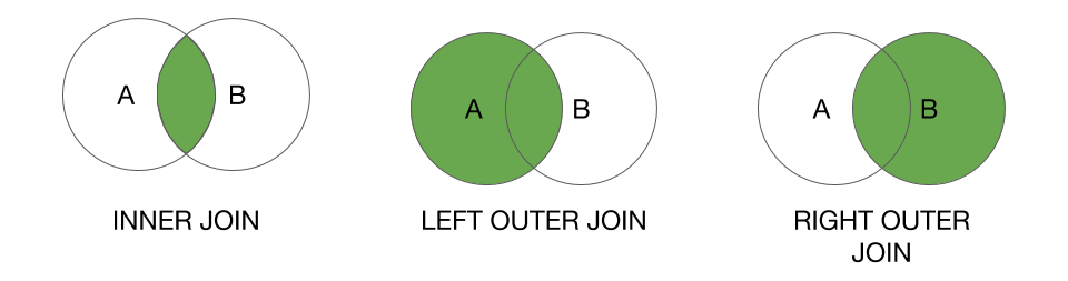
Join types

SQL Join Type	In Spark (synonyms)	Description
INNER	"inner"	Data from left and right matching both ways (intersection)
FULL OUTER	"outer", "full", "fullouter"	All rows from left and right with extra data if present (union)
LEFT OUTER	"leftouter", "left"	Rows from left with extra data from right if present
RIGHT OUTER	"rightouter", "right"	Rows from right with extra data from left if present
LEFT SEMI	"leftsemi"	Data from left with a match with right
LEFT ANTI	"leftanti"	Data from left with no match with right
CROSS	"cross"	Cartesian product of left and right (never used)

Join types

Inner join (“inner”)

>>> inner = df_left.join(df_right, "id", "inner")

df_left                df_right             
+---+-----+            +---+-----+
| id|value|            | id|value|
+---+-----+            +---+-----+
|  1|   A1|            |  3|   A3|
|  2|   A2|            |  4| A4_1|
|  3|   A3|            |  4|   A4|
|  4|   A4|            |  5|   A5|
+---+-----+            |  6|   A6|
                       +---+-----+
inner
+---+-----+-----+
| id|value|value|
+---+-----+-----+
|  3|   A3|   A3|
|  4|   A4|   A4|
|  4|   A4| A4_1|
+---+-----+-----+

Outer join (“outer”, “full” or “fullouter”)

>>> outer = df_left.join(df_right, "id", "outer")
df_left                df_right             
+---+-----+            +---+-----+
| id|value|            | id|value|
+---+-----+            +---+-----+
|  1|   A1|            |  3|   A3|
|  2|   A2|            |  4| A4_1|
|  3|   A3|            |  4|   A4|
|  4|   A4|            |  5|   A5|
+---+-----+            |  6|   A6|
                       +---+-----+
outer
+---+-----+-----+
| id|value|value|
+---+-----+-----+
|  1|   A1| null|
|  2|   A2| null|
|  3|   A3|   A3|
|  4|   A4|   A4|
|  4|   A4| A4_1|
|  5| null|   A5|
|  6| null|   A6|
+---+-----+-----+

Left join (“leftouter” or “left” )

>>> left = df_left.join(df_right, "id", "left")

df_left                df_right             
+---+-----+            +---+-----+
| id|value|            | id|value|
+---+-----+            +---+-----+
|  1|   A1|            |  3|   A3|
|  2|   A2|            |  4| A4_1|
|  3|   A3|            |  4|   A4|
|  4|   A4|            |  5|   A5|
+---+-----+            |  6|   A6|
                       +---+-----+
left
+---+-----+-----+
| id|value|value|
+---+-----+-----+
|  1|   A1| null|
|  2|   A2| null|
|  3|   A3|   A3|
|  4|   A4|   A4|
|  4|   A4| A4_1|
+---+-----+-----+

Right (“rightouter” or “right”)

>>> right = df_left.join(df_right, "id", "right")

df_left                df_right             
+---+-----+            +---+-----+
| id|value|            | id|value|
+---+-----+            +---+-----+
|  1|   A1|            |  3|   A3|
|  2|   A2|            |  4| A4_1|
|  3|   A3|            |  4|   A4|
|  4|   A4|            |  5|   A5|
+---+-----+            |  6|   A6|
                       +---+-----+
right
+---+-----+-----+
| id|value|value|
+---+-----+-----+
|  3|   A3|   A3|
|  4|   A4|   A4|
|  4|   A4| A4_1|
|  5| null|   A5|
|  6| null|   A6|
+---+-----+-----+

Left semi join (“leftsemi”)

>>> left_semi = df_left.join(df_right, "id", "leftsemi")

df_left                df_right             
+---+-----+            +---+-----+
| id|value|            | id|value|
+---+-----+            +---+-----+
|  1|   A1|            |  3|   A3|
|  2|   A2|            |  4| A4_1|
|  3|   A3|            |  4|   A4|
|  4|   A4|            |  5|   A5|
+---+-----+            |  6|   A6|
                       +---+-----+
left_semi
+---+-----+
| id|value|
+---+-----+
|  3|   A3|
|  4|   A4|
+---+-----+

Left anti joint (“leftanti”)

>>> left_anti = df_left.join(df_right, "id", "leftanti")

df_left                df_right             
+---+-----+            +---+-----+
| id|value|            | id|value|
+---+-----+            +---+-----+
|  1|   A1|            |  3|   A3|
|  2|   A2|            |  4| A4_1|
|  3|   A3|            |  4|   A4|
|  4|   A4|            |  5|   A5|
+---+-----+            |  6|   A6|
                       +---+-----+
left_anti
+---+-----+
| id|value|
+---+-----+
|  1|   A1|
|  2|   A2|
+---+-----+

Performing joins

• Node-to-node communication strategy

• Per node computation strategy

Section *“How Spark Performs Joins”

From the Definitive Guide:

Spark approaches cluster communication in two different ways during joins.

It either incurs a shuffle join, which results in an all-to-all communication or a broadcast join.

The core foundation of our simplified view of joins is that in Spark you will have either a big table or a small table.

When you join a big table to another big table, you end up with a shuffle join

When you join a big table to another big table, you end up with a shuffle join

When you join a big table to a small table, you end up with a broadcast join

Aggregations

Performing aggregations

• Maybe the most used operations in SQL and Spark SQL

• Similar to SQL, we use "group by" to perform aggregations

• We usually can call the aggregation function just after groupBy
  Namely, we use groupBy().agg()

• Many aggregation functions in pyspark.sql.functions

• Some examples:

  • Numerical: fn.avg, fn.sum, fn.min, fn.max, etc.

  • General: fn.first, fn.last, fn.count, fn.countDistinct, etc.

Examples

from pyspark.sql import functions as fn

products = spark.createDataFrame([
        ('1', 'mouse', 'microsoft', 39.99),
        ('2', 'mouse', 'microsoft', 59.99),
        ('3', 'keyboard', 'microsoft', 59.99),
        ('4', 'keyboard', 'logitech', 59.99),
        ('5', 'mouse', 'logitech', 29.99),
    ], ['prod_id', 'prod_cat', 'prod_brand', 'prod_value'])

products.groupBy('prod_cat').avg('prod_value').show()

# Or
products.groupBy('prod_cat').agg(fn.avg('prod_value')).show()

+--------+-----------------+
|prod_cat|  avg(prod_value)|
+--------+-----------------+
|   mouse|43.32333333333333|
|keyboard|            59.99|
+--------+-----------------+

+--------+-----------------+
|prod_cat|  avg(prod_value)|
+--------+-----------------+
|   mouse|43.32333333333333|
|keyboard|            59.99|
+--------+-----------------+

Examples

from pyspark.sql import functions as fn

products.groupBy('prod_brand', 'prod_cat')\
        .agg(fn.avg('prod_value')).show()

+----------+--------+---------------+
|prod_brand|prod_cat|avg(prod_value)|
+----------+--------+---------------+
| microsoft|   mouse|          49.99|
| microsoft|keyboard|          59.99|
|  logitech|keyboard|          59.99|
|  logitech|   mouse|          29.99|
+----------+--------+---------------+

Examples

from pyspark.sql import functions as fn

products.groupBy('prod_brand').agg(
    fn.round(fn.avg('prod_value'), 1).alias('average'),
    fn.ceil(fn.sum('prod_value')).alias('sum'),
    fn.min('prod_value').alias('min')
).show()

+----------+-------+---+-----+
|prod_brand|average|sum|  min|
+----------+-------+---+-----+
| microsoft|   53.3|160|39.99|
|  logitech|   45.0| 90|29.99|
+----------+-------+---+-----+

Examples

# Using an SQL query
products.createOrReplaceTempView("products")

query = """
  SELECT
    prod_brand,
    round(avg(prod_value), 1) AS average,
    min(prod_value) AS min
  FROM products
  GROUP BY prod_brand
"""

spark.sql(query).show()

+----------+-------+-----+
|prod_brand|average|  min|
+----------+-------+-----+
| microsoft|   53.3|39.99|
|  logitech|   45.0|29.99|
+----------+-------+-----+

Window functions

Window (analytic) functions

• A very, very powerful feature

• They allow to solve complex problems

• ANSI SQL2003 allows for a window_clause in aggregate function calls, the addition of which makes those functions into window functions

• A good article about this feature is [here]

See also :

https://www.postgresql.org/docs/current/tutorial-window.html

A window function performs a calculation across a set of table rows that are somehow related to the current row. This is comparable to the type of calculation that can be done with an aggregate function. However, window functions do not cause rows to become grouped into a single output row like non-window aggregate calls would. Instead, the rows retain their separate identities. Behind the scenes, the window function is able to access more than just the current row of the query result.

Window functions

• It’s similar to aggregations, but the number of rows doesn’t change

• Instead, new columns are created, and the aggregated values are duplicated for values of the same “group”

• There are

  • “traditional” aggregations, such as min, max, avg, sum and
  • “special” types, such as lag, lead, rank

Numerical window functions

from pyspark.sql import Window
from pyspark.sql import functions as fn

# First, we create the Window definition
window = Window.partitionBy('prod_brand')

# Then, we can use "over" to aggregate on this window
avg = fn.avg('prod_value').over(window)

# Finally, we can it as a classical column
products.withColumn('avg_brand_value', fn.round(avg, 2)).show()

+-------+--------+----------+----------+---------------+
|prod_id|prod_cat|prod_brand|prod_value|avg_brand_value|
+-------+--------+----------+----------+---------------+
|      4|keyboard|  logitech|     59.99|          44.99|
|      5|   mouse|  logitech|     29.99|          44.99|
|      1|   mouse| microsoft|     39.99|          53.32|
|      2|   mouse| microsoft|     59.99|          53.32|
|      3|keyboard| microsoft|     59.99|          53.32|
+-------+--------+----------+----------+---------------+

Numerical window functions

from pyspark.sql import Window
from pyspark.sql import functions as fn

# The window can be defined on multiple columns
window = Window.partitionBy('prod_brand', 'prod_cat')

avg = fn.avg('prod_value').over(window)

products.withColumn('avg_value', fn.round(avg, 2)).show()

+-------+--------+----------+----------+---------+
|prod_id|prod_cat|prod_brand|prod_value|avg_value|
+-------+--------+----------+----------+---------+
|      4|keyboard|  logitech|     59.99|    59.99|
|      5|   mouse|  logitech|     29.99|    29.99|
|      3|keyboard| microsoft|     59.99|    59.99|
|      1|   mouse| microsoft|     39.99|    49.99|
|      2|   mouse| microsoft|     59.99|    49.99|
+-------+--------+----------+----------+---------+

Numerical window functions

from pyspark.sql import Window
from pyspark.sql import functions as fn

# Multiple windows can be defined
window1 = Window.partitionBy('prod_brand')
window2 = Window.partitionBy('prod_cat')

avg_brand = fn.avg('prod_value').over(window1)
avg_cat = fn.avg('prod_value').over(window2)

products \
  .withColumn('avg_by_brand', fn.round(avg_brand, 2)) \
  .withColumn('avg_by_cat', fn.round(avg_cat, 2)) \
  .show()

+-------+--------+----------+----------+------------+----------+
|prod_id|prod_cat|prod_brand|prod_value|avg_by_brand|avg_by_cat|
+-------+--------+----------+----------+------------+----------+
|      4|keyboard|  logitech|     59.99|       44.99|     59.99|
|      3|keyboard| microsoft|     59.99|       53.32|     59.99|
|      5|   mouse|  logitech|     29.99|       44.99|     43.32|
|      1|   mouse| microsoft|     39.99|       53.32|     43.32|
|      2|   mouse| microsoft|     59.99|       53.32|     43.32|
+-------+--------+----------+----------+------------+----------+

Lag and Lead

• lag and lead are special functions used over an ordered window

• They are used to take the “previous” and “next” value within the window

• Very useful in datasets with a date column for instance

Lag and Lead

purchases = spark.createDataFrame([
        (date(2017, 11, 1), 'mouse'),
        (date(2017, 11, 2), 'mouse'),
        (date(2017, 11, 4), 'keyboard'),
        (date(2017, 11, 6), 'keyboard'),
        (date(2017, 11, 9), 'keyboard'),
        (date(2017, 11, 12), 'mouse'),
        (date(2017, 11, 18), 'keyboard')
    ], ['date', 'prod_cat'])
purchases.show()

+----------+--------+
|      date|prod_cat|
+----------+--------+
|2017-11-01|   mouse|
|2017-11-02|   mouse|
|2017-11-04|keyboard|
|2017-11-06|keyboard|
|2017-11-09|keyboard|
|2017-11-12|   mouse|
|2017-11-18|keyboard|
+----------+--------+

Lag and Lead

window = Window.partitionBy('prod_cat').orderBy('date')

prev_purch = fn.lag('date', 1).over(window)
next_purch = fn.lead('date', 1).over(window)

purchases\
  .withColumn('prev', prev_purch)\
  .withColumn('next', next_purch)\
  .orderBy('prod_cat', 'date')\
  .show()

+----------+--------+----------+----------+
|      date|prod_cat|      prev|      next|
+----------+--------+----------+----------+
|2017-11-04|keyboard|      NULL|2017-11-06|
|2017-11-06|keyboard|2017-11-04|2017-11-09|
|2017-11-09|keyboard|2017-11-06|2017-11-18|
|2017-11-18|keyboard|2017-11-09|      NULL|
|2017-11-01|   mouse|      NULL|2017-11-02|
|2017-11-02|   mouse|2017-11-01|2017-11-12|
|2017-11-12|   mouse|2017-11-02|      NULL|
+----------+--------+----------+----------+

Rank, DenseRank and RowNumber

• Another set of useful “special” functions

• Also used on ordered windows

• They create a rank, or an order of the items within the window

Rank and RowNumber

contestants = spark.createDataFrame([
    ('veterans', 'John', 3000),
    ('veterans', 'Bob', 3200),
    ('veterans', 'Mary', 4000),
    ('young', 'Jane', 4000),
    ('young', 'April', 3100),
    ('young', 'Alice', 3700),
    ('young', 'Micheal', 4000)], 
  ['category', 'name', 'points']
)

contestants.show()

+--------+-------+------+
|category|   name|points|
+--------+-------+------+
|veterans|   John|  3000|
|veterans|    Bob|  3200|
|veterans|   Mary|  4000|
|   young|   Jane|  4000|
|   young|  April|  3100|
|   young|  Alice|  3700|
|   young|Micheal|  4000|
+--------+-------+------+

Rank and RowNumber

window = Window.partitionBy('category')\
        .orderBy(contestants.points.desc())

rank = fn.rank().over(window)
dense_rank = fn.dense_rank().over(window)
row_number = fn.row_number().over(window)

contestants\
        .withColumn('rank', rank)\
        .withColumn('dense_rank', dense_rank)\
        .withColumn('row_number', row_number)\
        .orderBy('category', fn.col('points').desc())\
        .show()

+--------+-------+------+----+----------+----------+
|category|   name|points|rank|dense_rank|row_number|
+--------+-------+------+----+----------+----------+
|veterans|   Mary|  4000|   1|         1|         1|
|veterans|    Bob|  3200|   2|         2|         2|
|veterans|   John|  3000|   3|         3|         3|
|   young|   Jane|  4000|   1|         1|         1|
|   young|Micheal|  4000|   1|         1|         2|
|   young|  Alice|  3700|   3|         2|         3|
|   young|  April|  3100|   4|         3|         4|
+--------+-------+------+----+----------+----------+

Writing dataframes

Writing dataframes

• Very similar to reading. Output formats are the same: csv, json, parquet, orc, jdbc, etc. Note that write is an action

• Instead of df.read.{source} use df.write.{target}

• Main option is mode with possible values:

  • "append": append contents of this DataFrame to existing data.
  • "overwrite": overwrite existing data
  • "error": throw an exception if data already exists
  • "ignore": silently ignore this operation if data already exists.

Example

products.write.csv('./products.csv')
products.write.mode('overwrite').parquet('./produits.parquet')
products.write.format('parquet').save('./produits_2.parquet')

Under the hood…

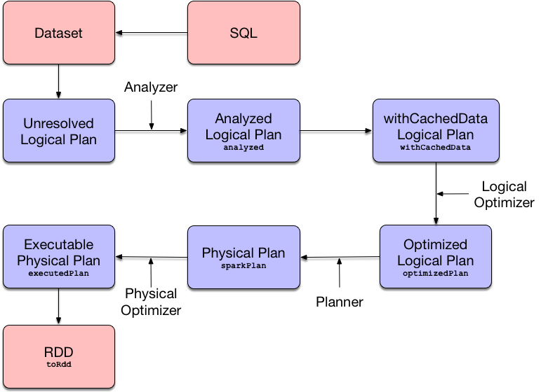
Query planning and optimization

A lot happens under the hood when executing an action on a DataFrame. The query goes through the following exectution stages:

1. Logical Analysis
2. Caching Replacement
3. Logical Query Optimization (using rule-based and cost-based optimizations)
4. Physical Planning
5. Physical Optimization (e.g. Whole-Stage Java Code Generation or Adaptive Query Execution)
6. Constructing the RDD of Internal Binary Rows (that represents the structured query in terms of Spark Core’s RDD API)

https://jaceklaskowski.gitbooks.io/mastering-spark-sql/spark-sql.html]

Query planning and optimization

https://jaceklaskowski.gitbooks.io/mastering-spark-sql/spark-sql.html]

References

PySpark Quickstart

Pandas on Spark User’s Guide

Thank you !