Introduction to `Pandas`

Pandas

Published

January 30, 2024

The Pandas library (https://Pandas.pydata.org) is one of the most popular tool for pythonistas dealing with data science.

It allows to crunch data easily
It mainly provides a DataFrame object (a table of data) with a huge set of functionalities

The Pandas book

Why ?

Through Pandas, you get acquainted with your data by analyzing them

What’s the average, median, max, or min of each column (statistical summaries)?
Does column A correlate with column B?
What does the distribution of data in column C look like?

Why (continued) ?

you first get acquainted with your data by cleaning and transforming

Pandas allows you to

Remove missing values, filter rows or/and columns
Store the cleaned, transformed data into virtually any format or database
Perform data visualization (when combined matplotlib, seaborn, plotly, …)

Where ?

Pandas is a central component of the python “stack” for data science

Pandas is built on top of numpy
often used in conjunction with other libraries
a DataFrame is often fed to plotting functions or machine learning algorithms (such as those provided by scikit-learn)
Pandas is well interfaced with jupyter, leading to a nice interactive environment for data exploration and modeling

Core components of Pandas

The two primary components of Pandas are Series and DataFrame.

A Series is essentially a column
A DataFrame is a two-dimensional table made up of a collection of Series with equal length

Note

According to Wes McKinney (the designer of Pandas) Pandas dataframes were inspired by dataframes offered by the R langugage for statistical computing. The latter parallels the tables that are at the heart of Relational Databases Management Systems.

Creating a `DataFrame` from scratch

import pandas as pd

fruits = {
    "apples": [3, 2, 0, 1],
    "oranges": [0, 3, 7, 2]
}

df_fruits = pd.DataFrame(fruits)
df_fruits

	apples	oranges
0	3	0
1	2	3
2	0	7
3	1	2

type(df_fruits)

pandas.core.frame.DataFrame

df_fruits["apples"]

0    3
1    2
2    0
3    1
Name: apples, dtype: int64

type(df_fruits["apples"])

pandas.core.series.Series

Note

Dataframes can be created in many different ways. Here we used a dictionary with values made of sequences of equal length. The dictionary keys serve as column names.

Common patterns of creation use Dataframe() from Pandas and call it with a list of dictionaries (each dictionary represents a row of the dataframe under construction) or a dictionary of lists/containers (as above).

Tidy dataframes

The notion of tidy dataframe has been popularized by Hadley Wickham. It embodies a collection of good practices that should be accepted by every data scientist.

A dataset is a collection of values, usually either numbers (if quantitative) or strings (if qualitative). Values are organised in two ways. Every value belongs to a variable and an observation. A variable contains all values that measure the same underlying attribute (like height, temperature, duration) across units. An observation contains all values measured on the same unit (like a person, or a day, or a race) across attributes.

Tidy data vignette

Datasets for fun

Your Pandas dataframes should abide.

tutorials = {
    "HS118": [
        "Getting Started With JupyterLab",
        "Introduction to Python for Scientific Programming",
        "Introduction to NumPy",
        "Introduction to pandas",
    ],
    "HS120": [
        "Increase Citations, Ease Review and Collaboration",
        "Time Series Forecasting With scikit-learn",
        "Evaluating Your Machine Learning Models",
        "Introduction to Audio and Speech Recognition",
    ],
}
schedule = pd.DataFrame(tutorials, index=["08:30", "10:30", "13:30", "15:30"])

schedule

	HS118	HS120
08:30	Getting Started With JupyterLab	Increase Citations, Ease Review and Collaboration
10:30	Introduction to Python for Scientific Programming	Time Series Forecasting With scikit-learn
13:30	Introduction to NumPy	Evaluating Your Machine Learning Models
15:30	Introduction to pandas	Introduction to Audio and Speech Recognition

Is it tidy? Why?

Pivot to long form using melt method

molten_schedule = schedule.melt(ignore_index=False)

What happens if we modify the optional argument ignore_index ?

(
    molten_schedule
      .reset_index()
      .rename(columns={
          "index": "time", 
          "variable": "room", 
          "value": "title"})
      .sort_values(by=["time", "room"])
      .reset_index(drop=True)
)

	time	room	title
0	08:30	HS118	Getting Started With JupyterLab
1	08:30	HS120	Increase Citations, Ease Review and Collaboration
2	10:30	HS118	Introduction to Python for Scientific Programming
3	10:30	HS120	Time Series Forecasting With scikit-learn
4	13:30	HS118	Introduction to NumPy
5	13:30	HS120	Evaluating Your Machine Learning Models
6	15:30	HS118	Introduction to pandas
7	15:30	HS120	Introduction to Audio and Speech Recognition

Index

At the end of the day, dataframes have to be queried, updated, just as tables in a RDBMS.

Every Pandas dataframe is equipped with an Index.

By default, a DataFrame uses a contiguous index
What if we want to know who buys the fruits ?

df_fruits = pd.DataFrame(fruits, index=["Daniel", "Sean", "Pierce", "Roger"])
df_fruits

	apples	oranges
Daniel	3	0
Sean	2	3
Pierce	0	7
Roger	1	2

Note

Is the index a column? How is it implemented?

Indexing using `.loc` versus `.iloc`

.loc locates by name
.iloc locates by numerical index (position)

df_fruits

	apples	oranges
Daniel	3	0
Sean	2	3
Pierce	0	7
Roger	1	2

# What's in Sean's basket ?
df_fruits.loc['Sean']

apples     2
oranges    3
Name: Sean, dtype: int64

# Who has oranges ?
df_fruits.loc[:, 'oranges']

Daniel    0
Sean      3
Pierce    7
Roger     2
Name: oranges, dtype: int64

# How many apples in Pierce's basket ?
df_fruits.loc['Pierce', 'apples']
df_fruits.loc['Sean', 'oranges']

df_fruits

	apples	oranges
Daniel	3	0
Sean	2	3
Pierce	0	7
Roger	1	2

df_fruits.iloc[2, 1]

Main attributes and methods of a `DataFrame`

A DataFrame has many attributes

df_fruits.columns

Index(['apples', 'oranges'], dtype='object')

df_fruits.index

Index(['Daniel', 'Sean', 'Pierce', 'Roger'], dtype='object')

df_fruits.dtypes

apples     int64
oranges    int64
dtype: object

A DataFrame has many methods

df_fruits.info()

<class 'pandas.core.frame.DataFrame'>
Index: 4 entries, Daniel to Roger
Data columns (total 2 columns):
 #   Column   Non-Null Count  Dtype
---  ------   --------------  -----
 0   apples   4 non-null      int64
 1   oranges  4 non-null      int64
dtypes: int64(2)
memory usage: 268.0+ bytes

df_fruits.describe()

	apples	oranges
count	4.000000	4.00000
mean	1.500000	3.00000
std	1.290994	2.94392
min	0.000000	0.00000
25%	0.750000	1.50000
50%	1.500000	2.50000
75%	2.250000	4.00000
max	3.000000	7.00000

Missing values

What if we don’t know how many apples are in Sean’s basket ?

df_fruits.loc['Sean', 'apples'] = None
df_fruits

	apples	oranges
Daniel	3.0	0
Sean	NaN	3
Pierce	0.0	7
Roger	1.0	2

df_fruits.describe()

	apples	oranges
count	3.000000	4.00000
mean	1.333333	3.00000
std	1.527525	2.94392
min	0.000000	0.00000
25%	0.500000	1.50000
50%	1.000000	2.50000
75%	2.000000	4.00000
max	3.000000	7.00000

Note that count is 3 for apples now, since we have 1 missing value among the 4

Adding a column

Ooooops, we forgot about the bananas !

df_fruits["bananas"] = [0, 2, 1, 6]
df_fruits

	apples	oranges	bananas
Daniel	3.0	0	0
Sean	NaN	3	2
Pierce	0.0	7	1
Roger	1.0	2	6

Adding a column with the date

And we forgot the dates !

df_fruits['time'] = [
    "2020/10/08 12:13", "2020/10/07 11:37", 
    "2020/10/10 14:07", "2020/10/09 10:51"
]
df_fruits

	apples	oranges	bananas	time
Daniel	3.0	0	0	2020/10/08 12:13
Sean	NaN	3	2	2020/10/07 11:37
Pierce	0.0	7	1	2020/10/10 14:07
Roger	1.0	2	6	2020/10/09 10:51

df_fruits.dtypes

apples     float64
oranges      int64
bananas      int64
time        object
dtype: object

type(df_fruits.loc["Roger", "time"])

str

It’s not a date but a string (str) ! So we convert this column to something called datetime

df_fruits["time"] = pd.to_datetime(df_fruits["time"])
df_fruits

	apples	oranges	bananas	time
Daniel	3.0	0	0	2020-10-08 12:13:00
Sean	NaN	3	2	2020-10-07 11:37:00
Pierce	0.0	7	1	2020-10-10 14:07:00
Roger	1.0	2	6	2020-10-09 10:51:00

df_fruits.dtypes

apples            float64
oranges             int64
bananas             int64
time       datetime64[ns]
dtype: object

What if we want to keep only the baskets after (including) October, 9th ?

df_fruits.loc[df_fruits["time"] >= pd.Timestamp("2020/10/09")]

	apples	oranges	bananas	time
Pierce	0.0	7	1	2020-10-10 14:07:00
Roger	1.0	2	6	2020-10-09 10:51:00

Date and time manipulation

Have a look at the documentation of the datetime package

https://docs.python.org/3/library/datetime.html

Slices and subsets of rows or columns

df_fruits

	apples	oranges	bananas	time
Daniel	3.0	0	0	2020-10-08 12:13:00
Sean	NaN	3	2	2020-10-07 11:37:00
Pierce	0.0	7	1	2020-10-10 14:07:00
Roger	1.0	2	6	2020-10-09 10:51:00

df_fruits.loc[:, "oranges":"time"]

	oranges	bananas	time
Daniel	0	0	2020-10-08 12:13:00
Sean	3	2	2020-10-07 11:37:00
Pierce	7	1	2020-10-10 14:07:00
Roger	2	6	2020-10-09 10:51:00

df_fruits.loc["Daniel":"Sean", "apples":"bananas"]

	apples	oranges	bananas
Daniel	3.0	0	0
Sean	NaN	3	2

df_fruits[["apples", "time"]]

	apples	time
Daniel	3.0	2020-10-08 12:13:00
Sean	NaN	2020-10-07 11:37:00
Pierce	0.0	2020-10-10 14:07:00
Roger	1.0	2020-10-09 10:51:00

Write our data to a CSV file

What if we want to write the file ?

df_fruits

	apples	oranges	bananas	time
Daniel	3.0	0	0	2020-10-08 12:13:00
Sean	NaN	3	2	2020-10-07 11:37:00
Pierce	0.0	7	1	2020-10-10 14:07:00
Roger	1.0	2	6	2020-10-09 10:51:00

df_fruits.to_csv("fruits.csv")

# Use !dir on windows
!ls -alh | grep fru

-rw-rw-r-- 1 boucheron boucheron  163 janv. 30 13:33 fruits.csv

!head -n 5 fruits.csv

,apples,oranges,bananas,time
Daniel,3.0,0,0,2020-10-08 12:13:00
Sean,,3,2,2020-10-07 11:37:00
Pierce,0.0,7,1,2020-10-10 14:07:00
Roger,1.0,2,6,2020-10-09 10:51:00

Warning

csv files are not the end of history.

They are not self-documented. They should be equiped with metadata.
There is no way to load a selection of columns,
csv have no built-in compression mechanism

The Apache arrow project offers a variety of file formats to remedy this set of drawbacks.

The DataFrame class is equipped with methods for saving to many formats.

[function for function in dir(pd.DataFrame) if function.startswith("to_")]

['to_clipboard',
 'to_csv',
 'to_dict',
 'to_excel',
 'to_feather',
 'to_gbq',
 'to_hdf',
 'to_html',
 'to_json',
 'to_latex',
 'to_markdown',
 'to_numpy',
 'to_orc',
 'to_parquet',
 'to_period',
 'to_pickle',
 'to_records',
 'to_sql',
 'to_stata',
 'to_string',
 'to_timestamp',
 'to_xarray',
 'to_xml']

Reading data and working with it

Let’s read the file tips.csv. It is a CSV file (Comma Separated Values).

It contains data about a restaurant: the bill, tip and some informations about the customers.

!ls

fruits.csv         notebook02_numpy.ipynb   notebook04_pandas.qmd
img            notebook02_numpy.qmd     tips.csv
miserable_word_counts.pkl  notebook03_pandas.ipynb
notebook01_python.qmd      notebook03_pandas.qmd

import requests
import os

# The path containing your notebook
path_data = './'
# The name of the file
filename = 'tips.csv'

if os.path.exists(os.path.join(path_data, filename)):
    print('The file %s already exists.' % os.path.join(path_data, filename))
else:
    url = 'http://stephane-v-boucheron.fr/data/tips.csv'
    r = requests.get(url)
    with open(os.path.join(path_data, filename), 'wb') as f:
        f.write(r.content)
    print(f'Downloaded file {os.path.join(path_data, filename)}.')

The file ./tips.csv already exists.

%ls -l *csv

-rw-rw-r-- 1 boucheron boucheron  163 janv. 30 13:33 fruits.csv
-rw-rw-r-- 1 boucheron boucheron 7943 janv. 29 22:13 tips.csv

df = pd.read_csv("tips.csv")

# `.head()` shows the first rows of the dataframe
df.head(n=10)

	total_bill	tip	sex	smoker	day	time	size
0	16.99	1.01	Female	No	Sun	Dinner	2
1	10.34	1.66	Male	No	Sun	Dinner	3
2	21.01	3.50	Male	No	Sun	Dinner	3
3	23.68	3.31	Male	No	Sun	Dinner	2
4	24.59	3.61	Female	No	Sun	Dinner	4
5	25.29	4.71	Male	No	Sun	Dinner	4
6	8.77	2.00	Male	No	Sun	Dinner	2
7	26.88	3.12	Male	No	Sun	Dinner	4
8	15.04	1.96	Male	No	Sun	Dinner	2
9	14.78	3.23	Male	No	Sun	Dinner	2

df.info()

<class 'pandas.core.frame.DataFrame'>
RangeIndex: 244 entries, 0 to 243
Data columns (total 7 columns):
 #   Column      Non-Null Count  Dtype  
---  ------      --------------  -----  
 0   total_bill  244 non-null    float64
 1   tip         244 non-null    float64
 2   sex         244 non-null    object 
 3   smoker      244 non-null    object 
 4   day         244 non-null    object 
 5   time        244 non-null    object 
 6   size        244 non-null    int64  
dtypes: float64(2), int64(1), object(4)
memory usage: 13.5+ KB

df.loc[42, "day"]

'Sun'

type(df.loc[42, "day"])

str

By default, columns that are non-numerical contain strings (str type)

The `category` type

An important type in Pandas is category for variables that are non-numerical

Pro tip. It’s always a good idea to tell Pandas which columns should be imported as categorical

So, let’s read again the file specifying some dtypes to the read_csv function

dtypes = {
    "sex": "category",
    "smoker": "category",
    "day": "category",
    "time": "category"
} 

df = pd.read_csv("tips.csv", dtype=dtypes)

df.dtypes

total_bill     float64
tip            float64
sex           category
smoker        category
day           category
time          category
size             int64
dtype: object

Important

Have a look at Pandas book on categorical datas

Computing statistics

# The describe method only shows statistics for the numerical columns by default
df.describe()

	total_bill	tip	size
count	244.000000	244.000000	244.000000
mean	19.785943	2.998279	2.569672
std	8.902412	1.383638	0.951100
min	3.070000	1.000000	1.000000
25%	13.347500	2.000000	2.000000
50%	17.795000	2.900000	2.000000
75%	24.127500	3.562500	3.000000
max	50.810000	10.000000	6.000000

# We use the include="all" option to see everything
df.describe(include="all")

	total_bill	tip	sex	smoker	day	time	size
count	244.000000	244.000000	244	244	244	244	244.000000
unique	NaN	NaN	2	2	4	2	NaN
top	NaN	NaN	Male	No	Sat	Dinner	NaN
freq	NaN	NaN	157	151	87	176	NaN
mean	19.785943	2.998279	NaN	NaN	NaN	NaN	2.569672
std	8.902412	1.383638	NaN	NaN	NaN	NaN	0.951100
min	3.070000	1.000000	NaN	NaN	NaN	NaN	1.000000
25%	13.347500	2.000000	NaN	NaN	NaN	NaN	2.000000
50%	17.795000	2.900000	NaN	NaN	NaN	NaN	2.000000
75%	24.127500	3.562500	NaN	NaN	NaN	NaN	3.000000
max	50.810000	10.000000	NaN	NaN	NaN	NaN	6.000000

# Correlation between the numerical columns
df.corr(numeric_only = True)

	total_bill	tip	size
total_bill	1.000000	0.675734	0.598315
tip	0.675734	1.000000	0.489299
size	0.598315	0.489299	1.000000

?df.corr

Data visualization with `matplotlib` and `seaborn`

Let’s show how we can use matplotlib and seaborn to visualize data contained in a Pandas dataframe

import matplotlib.pyplot as plt
import seaborn as sns

How do the tip depends on the total bill ?

sns.jointplot(x="total_bill", y="tip", data=df)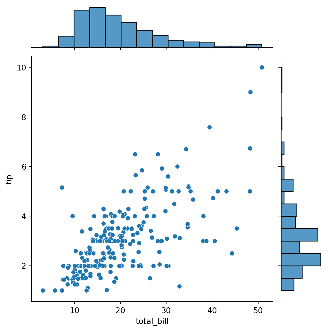

When do customers go to this restaurant ?

sns.countplot(x='day', hue="time", data=df)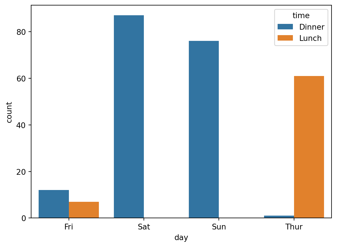

When do customers spend the most ?

plt.figure(figsize=(7, 5))
sns.boxplot(x='day', y='total_bill', hue='time', data=df)
plt.legend(loc="upper left")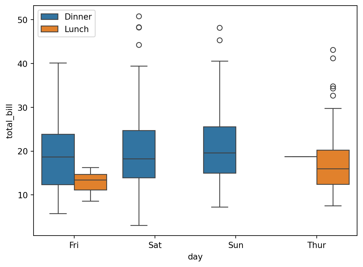

plt.figure(figsize=(7, 5))
sns.violinplot(x='day', y='total_bill', hue='time', split=True, data=df)
plt.legend(loc="upper left")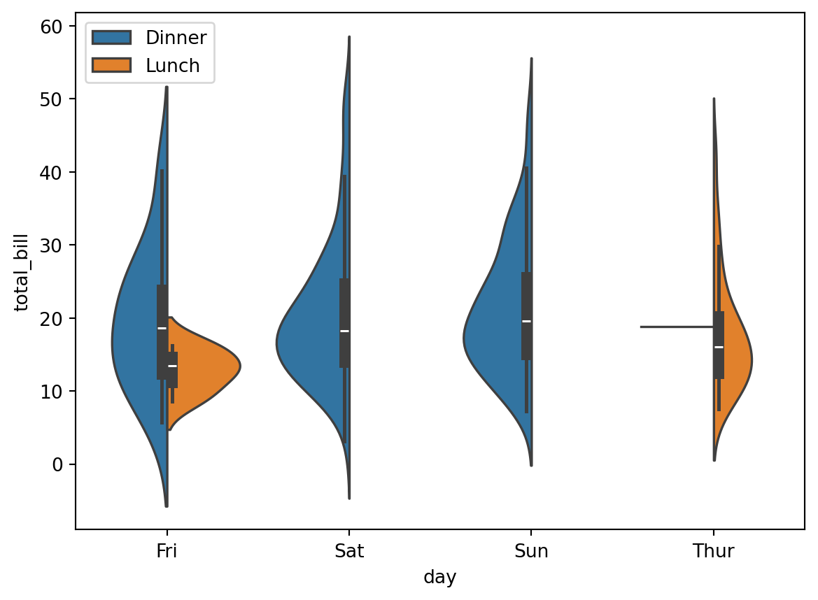

Who spends the most ?

sns.boxplot(x='sex', y='total_bill', hue='smoker', data=df)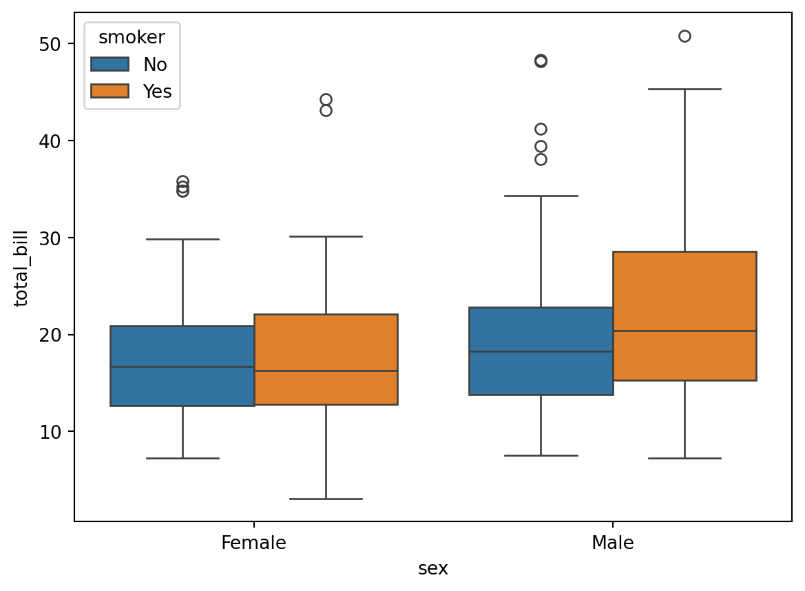

When should waiters want to work ?

sns.boxplot(x='day', y='tip', hue='time', data=df)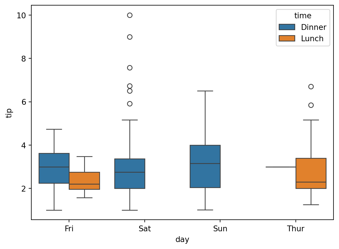

sns.violinplot(x='day', y='tip', hue='time', data=df)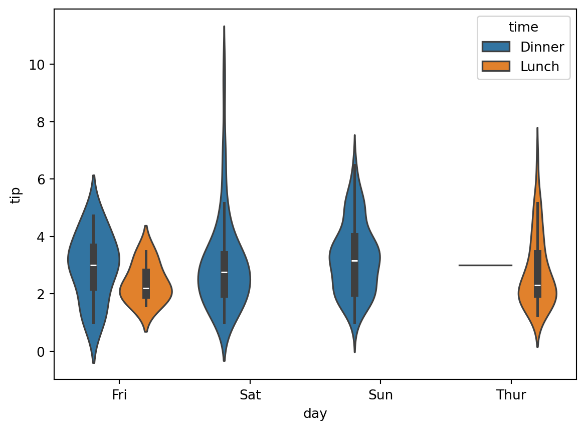

Data processing with `Pandas`

Let us read again the tips.csv file

import pandas as pd

dtypes = {
    "sex": "category",
    "smoker": "category",
    "day": "category",
    "time": "category"
} 

df = pd.read_csv("tips.csv", dtype=dtypes)
df.head()

	total_bill	tip	sex	smoker	day	time	size
0	16.99	1.01	Female	No	Sun	Dinner	2
1	10.34	1.66	Male	No	Sun	Dinner	3
2	21.01	3.50	Male	No	Sun	Dinner	3
3	23.68	3.31	Male	No	Sun	Dinner	2
4	24.59	3.61	Female	No	Sun	Dinner	4

Computations using `Pandas` : broadcasting

Let’s add a column that contains the tip percentage

df["tip_percentage"] = df["tip"] / df["total_bill"]
df.head()

	total_bill	tip	sex	smoker	day	time	size	tip_percentage
0	16.99	1.01	Female	No	Sun	Dinner	2	0.059447
1	10.34	1.66	Male	No	Sun	Dinner	3	0.160542
2	21.01	3.50	Male	No	Sun	Dinner	3	0.166587
3	23.68	3.31	Male	No	Sun	Dinner	2	0.139780
4	24.59	3.61	Female	No	Sun	Dinner	4	0.146808

The computation

df["tip"] / df["total_bill"]

uses a broadcast rule.

We can multiply, add, subtract, etc. together numpy arrays, Series or Pandas dataframes when the computation makes sense in view of their respective shape

This principle is called broadcast or broadcasting.

df["tip"].shape, df["total_bill"].shape

((244,), (244,))

The tip and total_billcolumns have the same shape, so broadcasting performs pairwise division.

This corresponds to the following “hand-crafted” approach with a for loop:

for i in range(df.shape[0]):
    df.loc[i, "tip_percentage"] = df.loc[i, "tip"] / df.loc[i, "total_bill"]

But using such a loop is:

much longer to write
prone to mistakes
ugly
and excruciatingly slower :(

NEVER use Python for-loops for numerical computations !

%%timeit -n 10
for i in range(df.shape[0]):
    df.loc[i, "tip_percentage"] = df.loc[i, "tip"] / df.loc[i, "total_bill"]

35.9 ms ± 1.92 ms per loop (mean ± std. dev. of 7 runs, 10 loops each)

%%timeit -n 10
df["tip_percentage"] = df["tip"] / df["total_bill"]

198 µs ± 27.5 µs per loop (mean ± std. dev. of 7 runs, 10 loops each)

The for loop is \(\approx\) 200 times slower ! (even worse on larger data)

Pitfall. Changing values in a `DataFrame`

When you want to change a value in a DataFrame, never use

df["tip_percentage"].loc[i] = 42

but use

df.loc[i, "tip_percentage"] = 42

namely, use a single loc or iloc statement. The first version might not work: it might modify a copy of the column and not the dataframe itself !

Another example of broadcasting is:

(100 * df[["tip_percentage"]]).head()

	tip_percentage
0	5.944673
1	16.054159
2	16.658734
3	13.978041
4	14.680765

where we multiplied each entry of the tip_percentage column by 100.

Remark. Note the difference between

df[['tip_percentage']]

which returns a DataFrame containing only the tip_percentage column and

df['tip_percentage']

which returns a Series containing the data of the tip_percentage column

Some more plots

How do the tip percentages relates to the total bill ?

sns.jointplot(x="total_bill", y="tip_percentage", data=df)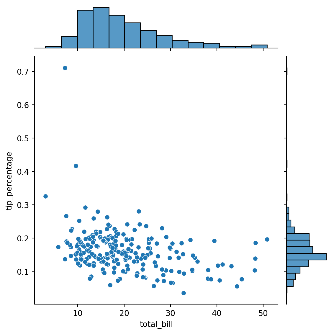

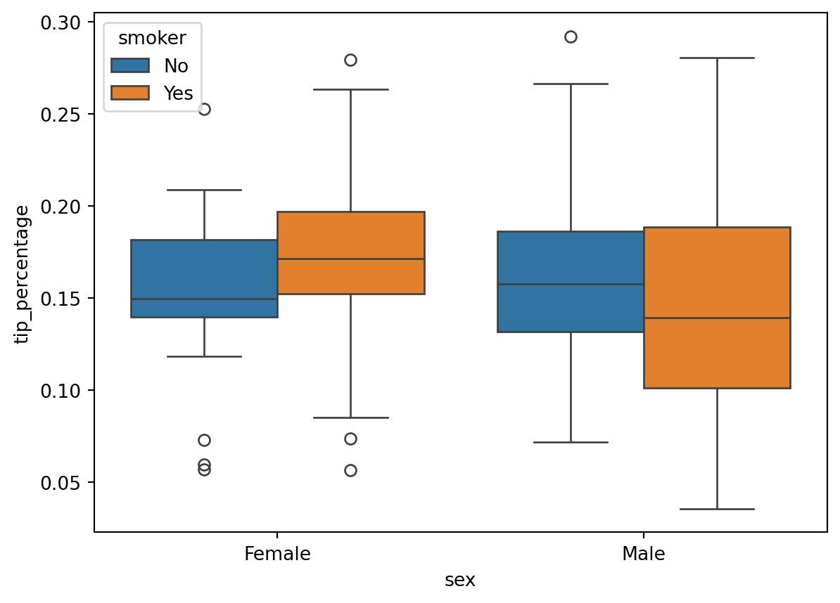
Who tips best ?

sns.boxplot(x='sex', y='tip_percentage', hue='smoker', data=df)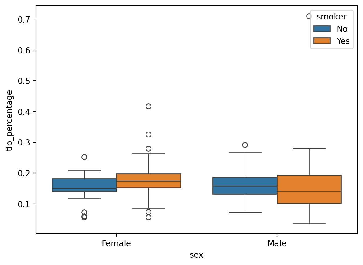

Who tips best without the `tip_percentage` outliers ?

sns.boxplot(
    x='sex', y='tip_percentage', hue='smoker', 
    data=df.loc[df["tip_percentage"] <= 0.3]
)

id(df)

139954175855872

The all-mighty `groupby` and `aggregate`

Many computations can be formulated as a groupby followed by and aggregation.

What is the mean `tip` and `tip percentage` each day ?

df.head()

	total_bill	tip	sex	smoker	day	time	size	tip_percentage
0	16.99	1.01	Female	No	Sun	Dinner	2	0.059447
1	10.34	1.66	Male	No	Sun	Dinner	3	0.160542
2	21.01	3.50	Male	No	Sun	Dinner	3	0.166587
3	23.68	3.31	Male	No	Sun	Dinner	2	0.139780
4	24.59	3.61	Female	No	Sun	Dinner	4	0.146808

df.groupby("day").mean()

/tmp/ipykernel_25457/381386936.py:1: FutureWarning:

The default of observed=False is deprecated and will be changed to True in a future version of pandas. Pass observed=False to retain current behavior or observed=True to adopt the future default and silence this warning.

TypeError: category dtype does not support aggregation 'mean'

But we don’t care about the size column here, so we can use insead

df[["total_bill", "tip", "tip_percentage", "day"]].groupby("day").mean()

/tmp/ipykernel_25457/1814539930.py:1: FutureWarning:

The default of observed=False is deprecated and will be changed to True in a future version of pandas. Pass observed=False to retain current behavior or observed=True to adopt the future default and silence this warning.

	total_bill	tip	tip_percentage
day
Fri	17.151579	2.734737	0.169913
Sat	20.441379	2.993103	0.153152
Sun	21.410000	3.255132	0.166897
Thur	17.682742	2.771452	0.161276

If we want to be more precise, we can groupby using several columns

(
    df[["total_bill", "tip", "tip_percentage", "day", "time"]]   # selection
        .groupby(["day", "time"])                                # partition
        .mean()                                                  # aggregation
)

/tmp/ipykernel_25457/125369857.py:3: FutureWarning:

The default of observed=False is deprecated and will be changed to True in a future version of pandas. Pass observed=False to retain current behavior or observed=True to adopt the future default and silence this warning.

		total_bill	tip	tip_percentage
day	time
Fri	Dinner	19.663333	2.940000	0.158916
Fri	Lunch	12.845714	2.382857	0.188765
Sat	Dinner	20.441379	2.993103	0.153152
Sat	Lunch	NaN	NaN	NaN
Sun	Dinner	21.410000	3.255132	0.166897
Sun	Lunch	NaN	NaN	NaN
Thur	Dinner	18.780000	3.000000	0.159744
Thur	Lunch	17.664754	2.767705	0.161301

Remarks

We obtain a DataFrame with a two-level indexing: on the day and the time
Groups must be homogeneous: we have NaN values for empty groups (e.g. Sat, Lunch)

Pro tip

Sometimes, it’s more convenient to get the groups as columns instead of a multi-level index.
For this, use reset_index:

(
    df[["total_bill", "tip", "tip_percentage", "day", "time"]]   # selection
        .groupby(["day", "time"])                                # partition
        .mean() # aggregation
        .reset_index()   # ako ungroup
)

/tmp/ipykernel_25457/835267922.py:3: FutureWarning:

The default of observed=False is deprecated and will be changed to True in a future version of pandas. Pass observed=False to retain current behavior or observed=True to adopt the future default and silence this warning.

	day	time	total_bill	tip	tip_percentage
0	Fri	Dinner	19.663333	2.940000	0.158916
1	Fri	Lunch	12.845714	2.382857	0.188765
2	Sat	Dinner	20.441379	2.993103	0.153152
3	Sat	Lunch	NaN	NaN	NaN
4	Sun	Dinner	21.410000	3.255132	0.166897
5	Sun	Lunch	NaN	NaN	NaN
6	Thur	Dinner	18.780000	3.000000	0.159744
7	Thur	Lunch	17.664754	2.767705	0.161301

Another pro tip

Computations with Pandas can include many operations that are pipelined until the final computation.
Pipelining many operations is good practice and perfectly normal, but in order to make the code readable you can put it between parenthesis (python expression) as follows:

(
    df[["total_bill", "tip", "tip_percentage", "day", "time"]]
    .groupby(["day", "time"])
    .mean()
    .reset_index()
    # and on top of all this we sort the dataframe with respect 
    # to the tip_percentage
    .sort_values("tip_percentage")
)

/tmp/ipykernel_25457/45053252.py:3: FutureWarning:

The default of observed=False is deprecated and will be changed to True in a future version of pandas. Pass observed=False to retain current behavior or observed=True to adopt the future default and silence this warning.

	day	time	total_bill	tip	tip_percentage
2	Sat	Dinner	20.441379	2.993103	0.153152
0	Fri	Dinner	19.663333	2.940000	0.158916
6	Thur	Dinner	18.780000	3.000000	0.159744
7	Thur	Lunch	17.664754	2.767705	0.161301
4	Sun	Dinner	21.410000	3.255132	0.166897
1	Fri	Lunch	12.845714	2.382857	0.188765
3	Sat	Lunch	NaN	NaN	NaN
5	Sun	Lunch	NaN	NaN	NaN

Displaying a `DataFrame` with `style`

Now, we can answer, with style, to the question: what are the average tip percentages along the week ?

(
    df[["tip_percentage", "day", "time"]]
    .groupby(["day", "time"])
    .mean()
    # At the end of the pipeline you can use .style
    .style
    # Print numerical values as percentages 
    .format("{:.2%}")
    .background_gradient()
)

/tmp/ipykernel_25457/838795167.py:3: FutureWarning:

The default of observed=False is deprecated and will be changed to True in a future version of pandas. Pass observed=False to retain current behavior or observed=True to adopt the future default and silence this warning.

ImportError: Pandas requires version '3.1.2' or newer of 'jinja2' (version '3.0.3' currently installed).

Removing the `NaN` values

But the NaN values are somewhat annoying. Let’s remove them

(
    df[["tip_percentage", "day", "time"]]
    .groupby(["day", "time"])
    .mean()
    # We just add this from the previous pipeline
    .dropna()
    .style
    .format("{:.2%}")
    .background_gradient()
)

/tmp/ipykernel_25457/2662169510.py:3: FutureWarning:

The default of observed=False is deprecated and will be changed to True in a future version of pandas. Pass observed=False to retain current behavior or observed=True to adopt the future default and silence this warning.

ImportError: Pandas requires version '3.1.2' or newer of 'jinja2' (version '3.0.3' currently installed).

Now, we clearly see when tip_percentage is maximal. But what about the standard deviation ?

We used only .mean() for now, but we can use several aggregating function using .agg()

(
    df[["tip_percentage", "day", "time"]]
    .groupby(["day", "time"])
    .agg(["mean", "std"])          # we feed `agg`  with a list of names of callables 
    .dropna()
    .style
    .format("{:.2%}")
    .background_gradient()
)

/tmp/ipykernel_25457/1856885208.py:3: FutureWarning:

The default of observed=False is deprecated and will be changed to True in a future version of pandas. Pass observed=False to retain current behavior or observed=True to adopt the future default and silence this warning.

ImportError: Pandas requires version '3.1.2' or newer of 'jinja2' (version '3.0.3' currently installed).

And we can use also .describe() as aggregation function. Moreover we - use the subset option to specify which column we want to style - we use ("tip_percentage", "count") to access multi-level index

(
    df[["tip_percentage", "day", "time"]]
    .groupby(["day", "time"])
    .describe()    # all-purpose summarising function
)

/tmp/ipykernel_25457/3924876303.py:3: FutureWarning:

The default of observed=False is deprecated and will be changed to True in a future version of pandas. Pass observed=False to retain current behavior or observed=True to adopt the future default and silence this warning.

		tip_percentage
		count	mean	std	min	25%	50%	75%	max
day	time
Fri	Dinner	12.0	0.158916	0.047024	0.103555	0.123613	0.144742	0.179199	0.263480
Fri	Lunch	7.0	0.188765	0.045885	0.117735	0.167289	0.187735	0.210996	0.259314
Sat	Dinner	87.0	0.153152	0.051293	0.035638	0.123863	0.151832	0.188271	0.325733
Sun	Dinner	76.0	0.166897	0.084739	0.059447	0.119982	0.161103	0.187889	0.710345
Thur	Dinner	1.0	0.159744	NaN	0.159744	0.159744	0.159744	0.159744	0.159744
Thur	Lunch	61.0	0.161301	0.038972	0.072961	0.137741	0.153846	0.193424	0.266312

(
    df[["tip_percentage", "day", "time"]]
    .groupby(["day", "time"])
    .describe()
    .dropna()
    .style
    .bar(subset=[("tip_percentage", "count")])
    .background_gradient(subset=[("tip_percentage", "50%")])
)

/tmp/ipykernel_25457/673231177.py:3: FutureWarning:

The default of observed=False is deprecated and will be changed to True in a future version of pandas. Pass observed=False to retain current behavior or observed=True to adopt the future default and silence this warning.

ImportError: Pandas requires version '3.1.2' or newer of 'jinja2' (version '3.0.3' currently installed).

Supervised learning of `tip` based on the `total_bill`

As an example of very simple machine-learning problem, let’s try to understand how we can predict tip based on total_bill.

import numpy as np

plt.scatter(df["total_bill"], df["tip"])
plt.xlabel("total_bill", fontsize=12)
plt.ylabel("tip", fontsize=12)

Text(0, 0.5, 'tip')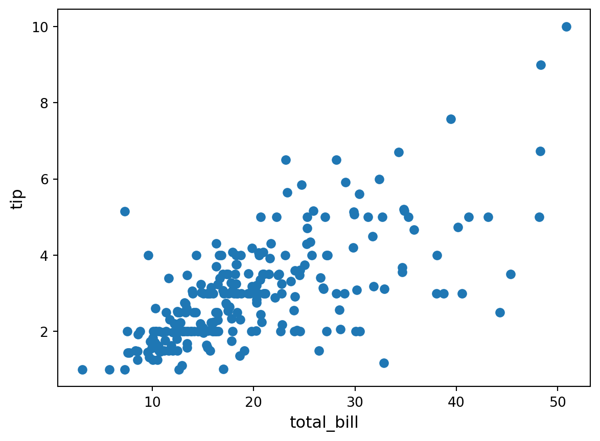

There’s a rough linear dependence between the two. Let’s try to find it by hand!
Namely, we look for numbers \(b\) and \(w\) such that

\[ \texttt{tip} \approx b + w \times \texttt{total_bill} \]

for all the examples of pairs of \((\texttt{tip}, \texttt{total_bill})\) we observe in the data.

In machine learning, we say that this is a very simple example of a supervised learning problem (here it is a regression problem), where \(\texttt{tip}\) is the label and where \(\texttt{total_bill}\) is the (only) feature, for which we intend to use a linear predictor.

plt.scatter(df["total_bill"], df["tip"])
plt.xlabel("total_bill", fontsize=12)
plt.ylabel("tip", fontsize=12)

slope = 1.0
intercept = 0.0

x = np.linspace(0, 50, 1000)
plt.plot(x, intercept + slope * x, color="red")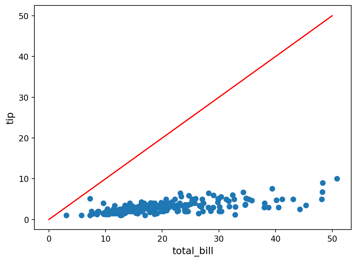

A more interactive way

This might require

# !pip install ipympl

import ipywidgets as widgets
import matplotlib.pyplot as plt
import numpy as np

%matplotlib widget
%matplotlib inline

x = np.linspace(0, 50, 1000)

@widgets.interact(intercept=(-5, 5, 1.), slope=(0, 1, .05))
def update(intercept=0.0, slope=0.5):
    plt.scatter(df["total_bill"], df["tip"])
    plt.plot(x, intercept + slope * x, color="red")
    plt.xlim((0, 50))
    plt.ylim((0, 10))
    plt.xlabel("total_bill", fontsize=12)
    plt.ylabel("tip", fontsize=12)

This is kind of tedious to do this by hand… it would be nice to come up with an automated way of doing this. Moreover:

We are using a linear function, while something more complicated (such as a polynomial) might be better
More importantly, we use only the total_bill column to predict the tip, while we know about many other things

df.head()

	total_bill	tip	sex	smoker	day	time	size	tip_percentage
0	16.99	1.01	Female	No	Sun	Dinner	2	0.059447
1	10.34	1.66	Male	No	Sun	Dinner	3	0.160542
2	21.01	3.50	Male	No	Sun	Dinner	3	0.166587
3	23.68	3.31	Male	No	Sun	Dinner	2	0.139780
4	24.59	3.61	Female	No	Sun	Dinner	4	0.146808

One-hot encoding of categorical variables

We can’t perform computations (products and sums) with columns containing categorical variables. So, we can’t use them like this to predict the tip. We need to convert them to numbers somehow.

The most classical approach for this is one-hot encoding (or “create dummies” or “binarize”) of the categorical variables, which can be easily achieved with Pandas.get_dummies

Why one-hot ? See wikipedia for a plausible explanation

df_one_hot = pd.get_dummies(df, prefix_sep='#')
df_one_hot.head(5)

	total_bill	tip	size	tip_percentage	sex#Female	sex#Male	smoker#No	smoker#Yes	day#Fri	day#Sat	day#Sun	day#Thur	time#Dinner	time#Lunch
0	16.99	1.01	2	0.059447	True	False	True	False	False	False	True	False	True	False
1	10.34	1.66	3	0.160542	False	True	True	False	False	False	True	False	True	False
2	21.01	3.50	3	0.166587	False	True	True	False	False	False	True	False	True	False
3	23.68	3.31	2	0.139780	False	True	True	False	False	False	True	False	True	False
4	24.59	3.61	4	0.146808	True	False	True	False	False	False	True	False	True	False

Only the categorical columns have been one-hot encoded. For instance, the "day" column is replaced by 4 columns named "day#Thur", "day#Fri", "day#Sat", "day#Sun", since "day" has 4 modalities (see next line).

df['day'].unique()

['Sun', 'Sat', 'Thur', 'Fri']
Categories (4, object): ['Fri', 'Sat', 'Sun', 'Thur']

df_one_hot.dtypes

total_bill        float64
tip               float64
size                int64
tip_percentage    float64
sex#Female           bool
sex#Male             bool
smoker#No            bool
smoker#Yes           bool
day#Fri              bool
day#Sat              bool
day#Sun              bool
day#Thur             bool
time#Dinner          bool
time#Lunch           bool
dtype: object

Pitfall. Colinearities with one-hot encoding

Sums over dummies for sex, smoker, day, time and size are all equal to one (by constrution of the one-hot encoded vectors).

Leads to colinearities in the matrix of features
It is much harder to train a linear regressor when the columns of the features matrix has colinearities

day_cols = [col for col in df_one_hot.columns if col.startswith("day")]
df_one_hot[day_cols].head()
df_one_hot[day_cols].sum(axis=1)

0      1
1      1
2      1
3      1
4      1
      ..
239    1
240    1
241    1
242    1
243    1
Length: 244, dtype: int64

all(df_one_hot[day_cols].sum(axis=1) == 1)

True

The most standard solution is to remove a modality (i.e. remove a one-hot encoding vector). Simply achieved by specifying drop_first=True in the get_dummies function.

df["day"].unique()

['Sun', 'Sat', 'Thur', 'Fri']
Categories (4, object): ['Fri', 'Sat', 'Sun', 'Thur']

pd.get_dummies(df, prefix_sep='#', drop_first=True).head()

	total_bill	tip	size	tip_percentage	sex#Male	smoker#Yes	day#Sat	day#Sun	day#Thur	time#Lunch
0	16.99	1.01	2	0.059447	False	False	False	True	False	False
1	10.34	1.66	3	0.160542	True	False	False	True	False	False
2	21.01	3.50	3	0.166587	True	False	False	True	False	False
3	23.68	3.31	2	0.139780	True	False	False	True	False	False
4	24.59	3.61	4	0.146808	False	False	False	True	False	False

Now, if a categorical feature has \(K\) modalities, we use only \(K-1\) dummies. For instance, there is no more sex#Female binary column.

Question. So, a linear regression won’t fit a weight for sex#Female. But, where do the model weights of the dropped binary columns go ?

Answer. They just “go” to the intercept: interpretation of the population bias depends on the “dropped” one-hot encodings.

So, we actually fit

\[ \begin{array}{rl} \texttt{tip} \approx b &+ w_1 \times \texttt{total_bill} + w_2 \times \texttt{size} \\ &+ w_3 \times \texttt{sex#Male} + w_4 \times \texttt{smoker#Yes} \\ &+ w_5 \times \texttt{day#Sat} + w_6 \times \texttt{day#Sun} + w_7 \times \texttt{day#Thur} \\ &+ w_8 \times \texttt{time#Lunch} \end{array} \]

Read the docs!

Why ?

Why (continued) ?

Where ?

Core components of Pandas

Creating a DataFrame from scratch

Tidy dataframes

Index

Indexing using .loc versus .iloc

Main attributes and methods of a DataFrame

Missing values

Adding a column

Adding a column with the date

Slices and subsets of rows or columns

Write our data to a CSV file

Reading data and working with it

The category type

Computing statistics

Data visualization with matplotlib and seaborn

How do the tip depends on the total bill ?

When do customers go to this restaurant ?

When do customers spend the most ?

Who spends the most ?

When should waiters want to work ?

Data processing with Pandas

Computations using Pandas : broadcasting

Pitfall. Changing values in a DataFrame

Some more plots

How do the tip percentages relates to the total bill ?

Who tips best ?

Who tips best without the tip_percentage outliers ?

The all-mighty groupby and aggregate

What is the mean tip and tip percentage each day ?

Pro tip

Another pro tip

Displaying a DataFrame with style

Removing the NaN values

Supervised learning of tip based on the total_bill

A more interactive way

One-hot encoding of categorical variables

Pitfall. Colinearities with one-hot encoding

Creating a `DataFrame` from scratch

Indexing using `.loc` versus `.iloc`

Main attributes and methods of a `DataFrame`

The `category` type

Data visualization with `matplotlib` and `seaborn`

Data processing with `Pandas`

Computations using `Pandas` : broadcasting

Pitfall. Changing values in a `DataFrame`

Who tips best without the `tip_percentage` outliers ?

The all-mighty `groupby` and `aggregate`

What is the mean `tip` and `tip percentage` each day ?

Displaying a `DataFrame` with `style`

Removing the `NaN` values

Supervised learning of `tip` based on the `total_bill`