EDA IX: Hierarchical Clustering

.remark-slide-number .progress-bar-container {
  position: absolute;
  bottom: 0;
  height: 4px;
  display: block;
  left: 0;
  right: 0;
}

.remark-slide-number .progress-bar {
  height: 100%;
  background-color: red;
}
</style>

<div>
<style type="text/css">.xaringan-extra-logo {
width: 110px;
height: 128px;
z-index: 0;
background-image: url(./img/Universite_Paris_logo_horizontal.jpg);
background-size: contain;
background-repeat: no-repeat;
position: absolute;
top:1em;right:1em;
}
</style>
<script>(function () {
  let tries = 0
  function addLogo () {
    if (typeof slideshow === 'undefined') {
      tries += 1
      if (tries < 10) {
        setTimeout(addLogo, 100)
      }
    } else {
      document.querySelectorAll('.remark-slide-content:not(.hide_logo)')
        .forEach(function (slide) {
          const logo = document.createElement('a')
          logo.classList = 'xaringan-extra-logo'
          logo.href = 'http://master.math.univ-paris-diderot.fr/annee/m1-mi/'
          slide.appendChild(logo)
        })
    }
  }
  document.addEventListener('DOMContentLoaded', addLogo)
})()</script>
</div>

---
name: inter-slide
class: left, middle, inverse

---

# Exploratory Data Analysis : Hierarchical Clustering

### 2021-12-10

#### [Master I MIDS & MFA]()

#### [Analyse Exploratoire de Données](http://stephane-v-boucheron.fr/courses/eda/)

#### [Stéphane Boucheron](http://stephane-v-boucheron.fr)

---
exclude: true
template: inter-slide

# Exploratory Data Analysis IX Hierarchical Clustering

### 2021-12-10

#### [Master I MIDS & MFA]()

#### [Analyse Exploratoire de Données](http://stephane-v-boucheron.fr/courses/eda/)

#### [Stéphane Boucheron](http://stephane-v-boucheron.fr)

---
template: inter-slide

## <svg aria-hidden="true" role="img" viewBox="0 0 576 512" style="height:1em;width:1.12em;vertical-align:-0.125em;margin-left:auto;margin-right:auto;font-size:inherit;fill:white;overflow:visible;position:relative;"><path d="M0 117.66v346.32c0 11.32 11.43 19.06 21.94 14.86L160 416V32L20.12 87.95A32.006 32.006 0 0 0 0 117.66zM192 416l192 64V96L192 32v384zM554.06 33.16L416 96v384l139.88-55.95A31.996 31.996 0 0 0 576 394.34V48.02c0-11.32-11.43-19.06-21.94-14.86z"/></svg>

### [Hierarchical Clustering: the idea](#bigpic)

### [Inside `hclust`](#hclust)

### [Comparing dendrograms](#bla)

---
template: inter-slide
name: bigpic

## Hierarchical clustering

???

- Dendrogram : what is it?

- From dendrogram to clusterings: cutting a dendrogram

- Grow a dendrogram

- Displaying a dendrogram

- Validation and assesment

---

> Hierarchical clustering [...] is a method of cluster analysis which seeks to build a hierarchy of clusters

.fr.f6[Wikipedia]

Recall that a clustering is a _partition_ of some dataset

A partition `$D$` of `$\mathcal{X}$` is a _refinement_ of another partition `$D'$`
if every class in `$D$` is a subset of a class in `$D'$`. Partitions `$D$` and `$D'$` are
said to be _nested_

A hierarchical clustering of `$\mathcal{X}$` is a sequence of  `$|\mathcal{X}| -1$` nested partitions  of `$\mathcal{X}$`, starting from the trivial partition into  `$|\mathcal{X}|$` singletons and ending  into the trivial partition in `$1$` subset ( `$\mathcal{X}$` itself)

A hierarchical clustering consists of `$|\mathcal{X}|-1$` nested flat clusterings

We will explore _agglomerative_ or _bottom-up_ methods to build hierarchical clusterings

---

### Hierchical clustering and dendrograms

.fl.w-40.f6.pa2[

The result of hierarchical clustering is a tree where leafs are labelled by sample points and
internal nodes correspond to merging operations

The tree conveys more information: if the tree is properly decorated, it is possible to reconstruct the different merging steps and to know which rule was applied when some merging operation was performed

The tree is called a _dendrogram_

]

.fl.w-60.pa2[

]

???

Dendrogram and trees show up in several areas.

Classification and Regression trees play an important role in Machine Learning.

`ggdendro` and `dendextend`  may also be used to manipulate regression trees

---

### <svg aria-hidden="true" role="img" viewBox="0 0 512 512" style="height:1em;width:1em;vertical-align:-0.125em;margin-left:auto;margin-right:auto;font-size:inherit;fill:currentColor;overflow:visible;position:relative;"><path d="M416 320h-96c-17.6 0-32-14.4-32-32s14.4-32 32-32h96s96-107 96-160-43-96-96-96-96 43-96 96c0 25.5 22.2 63.4 45.3 96H320c-52.9 0-96 43.1-96 96s43.1 96 96 96h96c17.6 0 32 14.4 32 32s-14.4 32-32 32H185.5c-16 24.8-33.8 47.7-47.3 64H416c52.9 0 96-43.1 96-96s-43.1-96-96-96zm0-256c17.7 0 32 14.3 32 32s-14.3 32-32 32-32-14.3-32-32 14.3-32 32-32zM96 256c-53 0-96 43-96 96s96 160 96 160 96-107 96-160-43-96-96-96zm0 128c-17.7 0-32-14.3-32-32s14.3-32 32-32 32 14.3 32 32-14.3 32-32 32z"/></svg>

- Cutting a dendrogram: getting a flat clustering

- Building a dendrogram: inside `hclust`

- Displaying, reporting dendrograms

---

### Cutting a dendrogram: Iris illustration

> The famous (Fisher’s or Anderson’s) iris data set gives the measurements in centimeters of the variables sepal length and width and petal length and width, respectively, for 50 flowers from each of 3 species of iris. The species are Iris setosa, versicolor, and virginica.

.fr.f6[[From `?iris`] ]

> The Iris flower data set is fun for learning supervised classification algorithms, and is known as a difficult case for unsupervised learning.

> The Setosa species are distinctly different from Versicolor and Virginica (they have lower petal length and width). But Versicolor and Virginica cannot easily be separated based on measurements of their sepal and petal width/length.

.fr.f6[[From `dendextend ` package]]

]

```r
iris_num <- select(iris, where(is.numeric))
rownames(iris_num) <- str_c(iris$Species,
                            1:150, sep = "_")

iris_num %>%
* dist() %>%
* hclust() ->  iris_hclust

*iris_dendro <- dendro_data(iris_hclust)

*ggdendrogram(iris_dendro,
            leaf_labels = TRUE,
            rotate = TRUE) +
  ggtitle("Dendrogram for Iris") +
  theme_dendro() +
#  coord_flip() +
  scale_y_reverse(expand = c(0.2, 0))
```

```
## Scale for 'y' is already present. Adding another scale for 'y', which will
## replace the existing scale.
```
]

]

???

- `as.matrix(dist(iris[,1:4]))` returns the matrix of pairwise distances
- default distance is Euclidean distance
- Using `broom::augment` ??
- There is no `augment.hclust` method: `No augment method for objects of class hclust`

- Plot comments

---
exclude: true

### Inside ggdendro

```r
hc <- hclust(dist(iris[,1:4]), "ave")
hcdata <- dendro_data(hc, type = "rectangle")
ggplot() +
* geom_segment(data = segment(hcdata),
               aes(x = x, y = y, xend = xend, yend = yend)
  ) +
* geom_text(data = label(hcdata),
            aes(x = x, y = y, label = label, hjust = 0),
            size = 2
  ) +
  coord_flip() +
  scale_y_reverse(expand = c(0.2, 0)) +
  theme_dendro()
```

---

### Cutting a dendrogram: <svg aria-hidden="true" role="img" viewBox="0 0 512 512" style="height:1em;width:1em;vertical-align:-0.125em;margin-left:auto;margin-right:auto;font-size:inherit;fill:currentColor;overflow:visible;position:relative;"><path d="M201.5 174.8l55.7 55.8c3.1 3.1 3.1 8.2 0 11.3l-11.3 11.3c-3.1 3.1-8.2 3.1-11.3 0l-55.7-55.8-45.3 45.3 55.8 55.8c3.1 3.1 3.1 8.2 0 11.3l-11.3 11.3c-3.1 3.1-8.2 3.1-11.3 0L111 265.2l-26.4 26.4c-17.3 17.3-25.6 41.1-23 65.4l7.1 63.6L2.3 487c-3.1 3.1-3.1 8.2 0 11.3l11.3 11.3c3.1 3.1 8.2 3.1 11.3 0l66.3-66.3 63.6 7.1c23.9 2.6 47.9-5.4 65.4-23l181.9-181.9-135.7-135.7-64.9 65zm308.2-93.3L430.5 2.3c-3.1-3.1-8.2-3.1-11.3 0l-11.3 11.3c-3.1 3.1-3.1 8.2 0 11.3l28.3 28.3-45.3 45.3-56.6-56.6-17-17c-3.1-3.1-8.2-3.1-11.3 0l-33.9 33.9c-3.1 3.1-3.1 8.2 0 11.3l17 17L424.8 223l17 17c3.1 3.1 8.2 3.1 11.3 0l33.9-34c3.1-3.1 3.1-8.2 0-11.3l-73.5-73.5 45.3-45.3 28.3 28.3c3.1 3.1 8.2 3.1 11.3 0l11.3-11.3c3.1-3.2 3.1-8.2 0-11.4z"/></svg> Iris illustration (continued)

```r
p <- iris %>%
  ggplot() +
  aes(x=Petal.Length, y=Petal.Width)

p +
  geom_point(aes(shape=Species)) +
  labs(shape= "Species") +
  ggtitle(label= "Iris data",
          subtitle = "Species in Petal plane")
```
]

![](cm-9-EDA_files/figure-html/iris-hclust-1-1.png)

]

???

Does the flat clustering obtained by cutting the dendrogram at some height
reflect the partition into species

---

### Cutting a dendrogram:  Iris illustration (continued)

```r
*iris_3 <- cutree(iris_hclust, 3)
p +
  geom_point(aes(shape=Species,
*                colour=factor(iris_3))) +
  labs(colour= "Clusters") +
  ggtitle("Iris data",
          "Hierarchical clustering, 3 classes")
```

]

![](cm-9-EDA_files/figure-html/iris-hclust-2-1.png)

]
]
---

### Cutting a dendrogram:  Iris illustration (continued)

```r
p +
  geom_point(aes(shape=Species,
                 colour=factor(iris_3))) +
  labs(colour= "Clusters") +
  labs(shape="Species") +
  ggtitle("Iris data",
          "Hierarchical clustering and Species")
```
]

![](cm-9-EDA_files/figure-html/iris-hclust-3-1.png)

]

---

### Cutting a dendrogram:  Iris illustration (continued)

```r
*iris_2 <- cutree(iris_hclust, 2)

p +
  geom_point(aes(shape=Species,
                 colour=factor(iris_2))) +
  labs(colour= "Clusters") +
  labs(shape="Species") +
  ggtitle("Iris data",
          "Clustering in 2 classes and Species")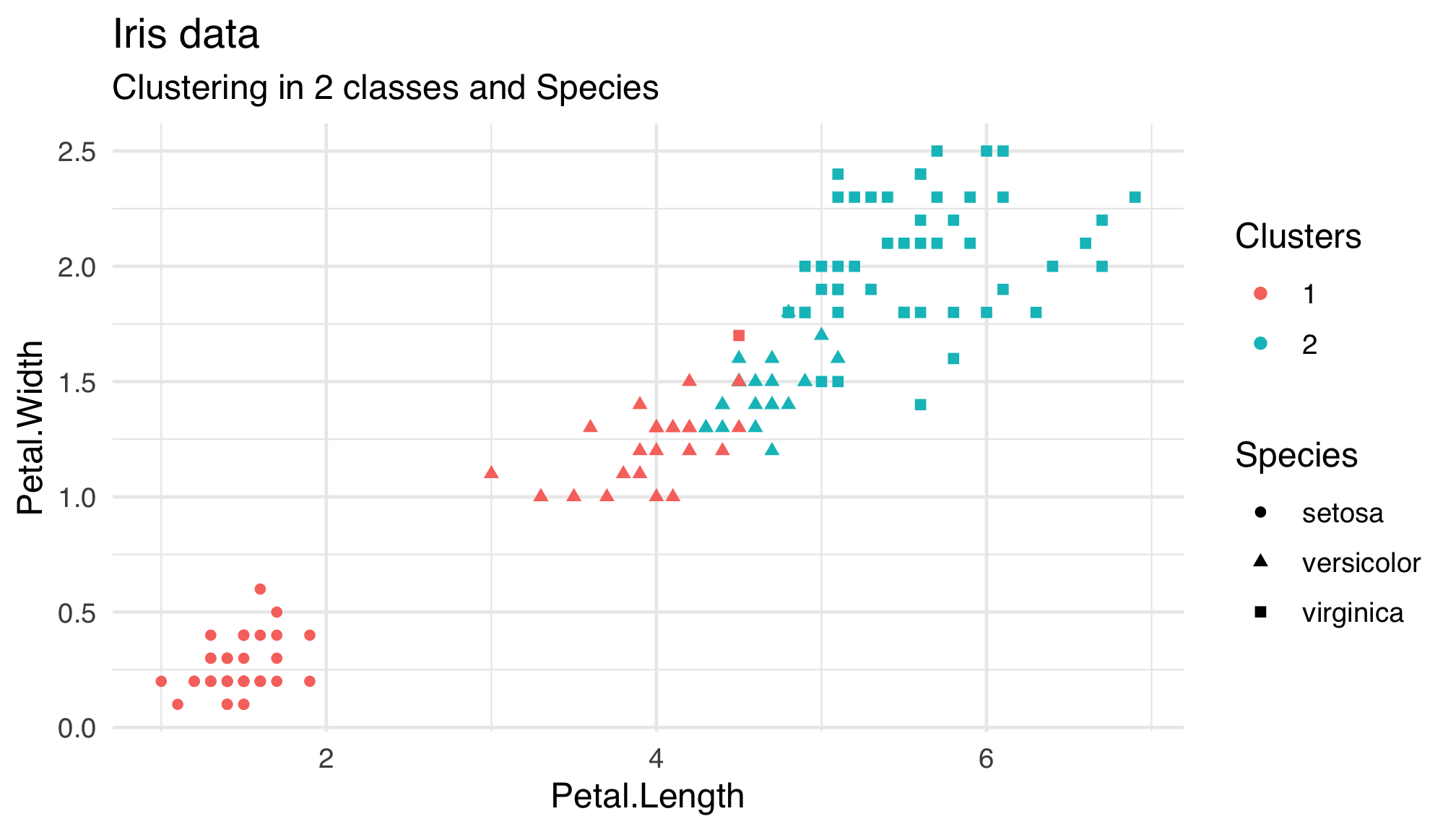
```
]

![](cm-9-EDA_files/figure-html/iris-hclust-4-1.png)

]

---

### Cutting a dendrogram:  Iris illustration (continued)

```r
*iris_4 <- cutree(iris_hclust, 4)

p +
  geom_point(aes(shape=Species,
                 colour=factor(iris_4))) +
  labs(colour= "Clusters") +
  labs(shape="Species") +
  ggtitle("Iris data",
          "Clustering in 4 classes and Species")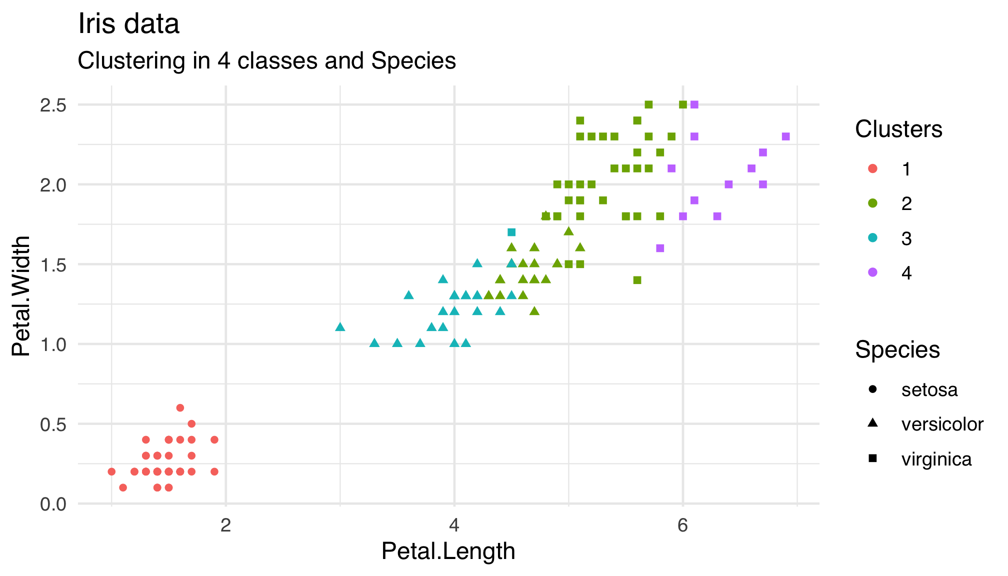
```
]

]

---
exclude: true

```r
sample_iris <-
  rownames_to_column(iris, var = "num") %>%
  group_by(Species) %>%
  sample_n(10)
```

---

### Cutting a dendrogram:  better Iris illustration (continued)

The [`dendextend`](https://talgalili.github.io/dendextend/articles/dendextend.html) package offers a set of functions for extending _dendrogram_ objects in <svg aria-hidden="true" role="img" viewBox="0 0 581 512" style="height:1em;width:1.13em;vertical-align:-0.125em;margin-left:auto;margin-right:auto;font-size:inherit;fill:currentColor;overflow:visible;position:relative;"><path d="M581 226.6C581 119.1 450.9 32 290.5 32S0 119.1 0 226.6C0 322.4 103.3 402 239.4 418.1V480h99.1v-61.5c24.3-2.7 47.6-7.4 69.4-13.9L448 480h112l-67.4-113.7c54.5-35.4 88.4-84.9 88.4-139.7zm-466.8 14.5c0-73.5 98.9-133 220.8-133s211.9 40.7 211.9 133c0 50.1-26.5 85-70.3 106.4-2.4-1.6-4.7-2.9-6.4-3.7-10.2-5.2-27.8-10.5-27.8-10.5s86.6-6.4 86.6-92.7-90.6-87.9-90.6-87.9h-199V361c-74.1-21.5-125.2-67.1-125.2-119.9zm225.1 38.3v-55.6c57.8 0 87.8-6.8 87.8 27.3 0 36.5-38.2 28.3-87.8 28.3zm-.9 72.5H365c10.8 0 18.9 11.7 24 19.2-16.1 1.9-33 2.8-50.6 2.9v-22.1z"/></svg>, letting you

- visualize and
- compare trees of hierarchical clusterings,

Features:

- Adjust a tree’s graphical parameters - the color, size, type, etc of its branches, nodes and labels
- Visually and statistically compare different dendrograms to one another

]

```r
require(dendextend)
require(colorspace)
species_col <- rev(rainbow_hcl(3))[as.numeric(iris$Species)]
*dend <- as.dendrogram(iris_hclust)

# order it the closest we can to the order of the observations:
dend <- rotate(dend, 1:150)

# Color the branches based on the clusters:
dend <- color_branches(dend, k=3) #, groupLabels=iris_species)

# Manually match the labels, as much as possible, to the real classification of the flowers:
labels_colors(dend) <-
   rainbow_hcl(3)[sort_levels_values(
      as.numeric(iris[,5])[order.dendrogram(dend)]
   )]
```

]

```r
# We hang the dendrogram a bit:
*dend <- hang.dendrogram(dend, hang_height=0.1)
# reduce the size of the labels:
*dend <- assign_values_to_leaves_nodePar(dend, 0.5, "lab.cex")
# dend <- set(dend, "labels_cex", 0.5)
# And plot:
par(mar = c(3,3,3,7))
plot(dend,
     main = "Clustered Iris data set
     (the labels give the true flower species)",
     horiz =  TRUE,  nodePar = list(cex = .007))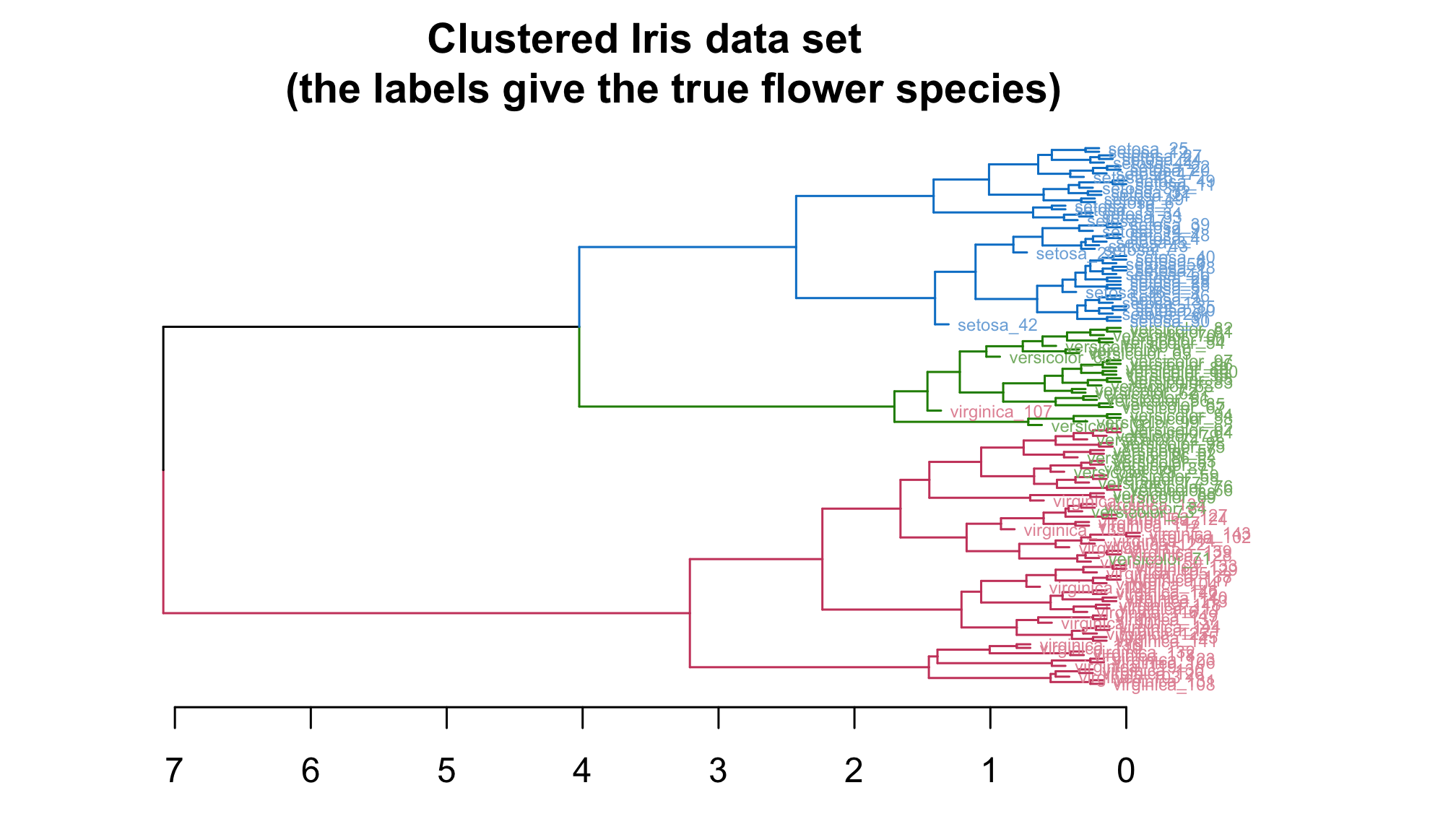
```

]

![](cm-9-EDA_files/figure-html/hang-iris-1.png)

]

]

???

- []()

- [dendextend](https://talgalili.github.io/dendextend/articles/dendextend.html)

- [A dendro gallery](https://www.r-graph-gallery.com/340-custom-your-dendrogram-with-dendextend.html)

- class of `dend`

---
template: inter-slide
name: hclust

## Inside `hclust`

---

### About class `hclust`

Results from function `hclust()` are objects of class `hclust` :

`iris_hclust` is an object of class hclust

Function `cutree()` returns a flat clustering of the dataset

???

What does `height` stand for?

What does `merge` stand for?

What does `order` stand for?

How different are the different `method`?

---

### Hierarchical clustering of `USArrests`

```r
data("USArrests")
USArrests %>% glimpse()
```

```
## Rows: 50
## Columns: 4
## $ Murder   <dbl> 13.2, 10.0, 8.1, 8.8, 9.0, 7.9, 3.3, 5.9, 15.4, 17.4, 5.3, 2.…
## $ Assault  <int> 236, 263, 294, 190, 276, 204, 110, 238, 335, 211, 46, 120, 24…
## $ UrbanPop <int> 58, 48, 80, 50, 91, 78, 77, 72, 80, 60, 83, 54, 83, 65, 57, 6…
## $ Rape     <dbl> 21.2, 44.5, 31.0, 19.5, 40.6, 38.7, 11.1, 15.8, 31.9, 25.8, 2…
```

]

```r
hc <- hclust(dist(scale(USArrests[,-3])), "ave")
*hcdata <- dendro_data(hc, type = "rectangle")

ggplot() +
  geom_segment(data = segment(hcdata),
               aes(x = x, y = y,
                   xend = xend, yend = yend)
  ) +
  geom_text(data = label(hcdata),
            aes(x = x, y = y,
                label = label, hjust = 0),
            size = 3
  ) +
  coord_flip() +
  scale_y_reverse(expand = c(0.2, 0))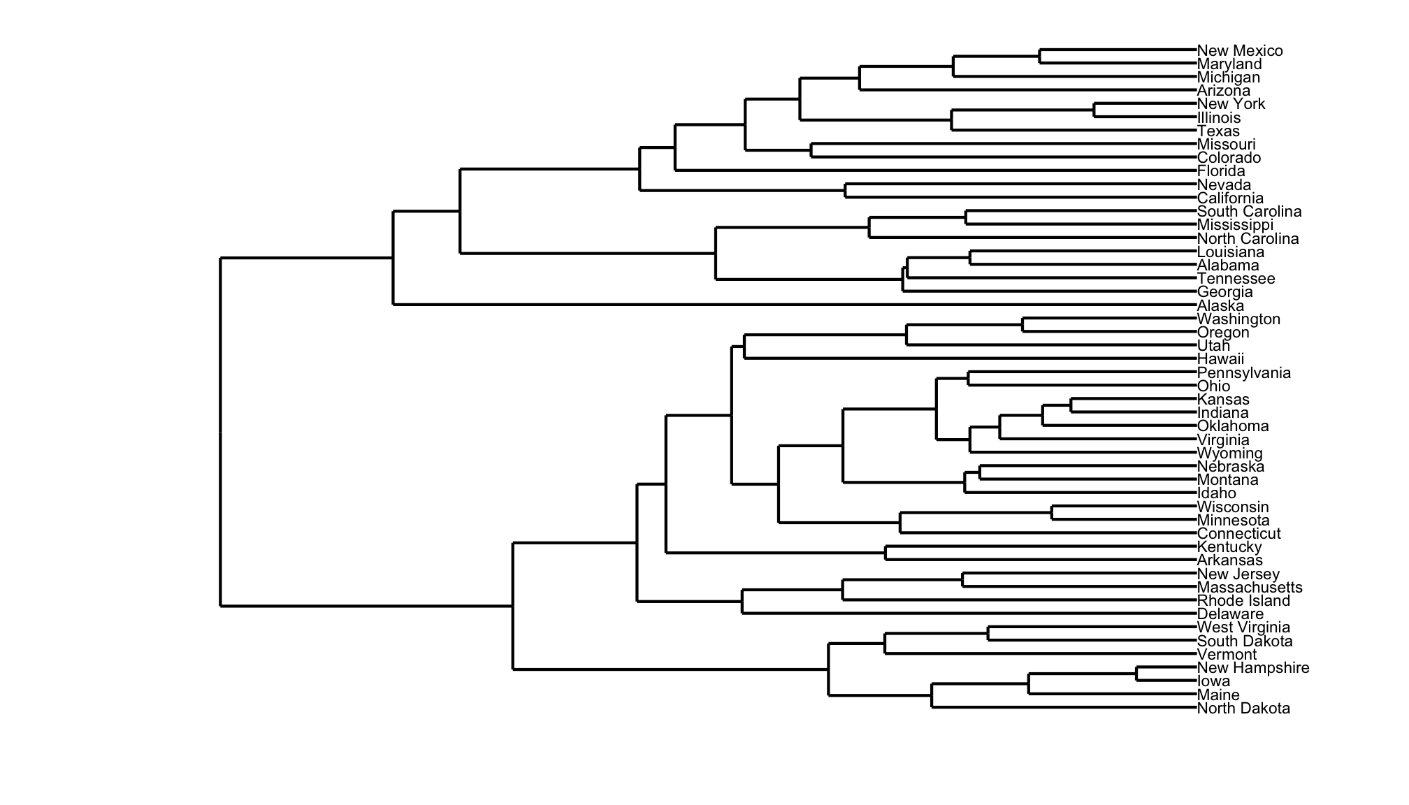
```
]

![](cm-9-EDA_files/figure-html/dendro-USArrests-1.png)

]

---

### About dendrograms

`iris_dendro` is an object of class dendro

An object of class `dendro` is a list of 4 objects:
  - `segments`
  - `labels`
  - `leaf_labels`
  - `class`

```r
iris_dendro <- dendro_data(iris_hclust)
```

???

dendrogram <-> `ultrametric` disimilarities

---

### Questions

- How to build the dendrogram?

- How to choose the cut?

---

### Bird-eye view at hierarchical agglomerative clustering methods

#### All [hierarchical agglomerative clustering methods (HACMs)](https://en.wikipedia.org/wiki/Hierarchical_clustering) can be described by the following general algorithm.

1. At each stage distances between clusters are recomputed by the _Lance-Williams dissimilarity update formula_ according to the particular clustering method being used.

1. Identify the 2 closest _points_ and combine them into a cluster (treating existing clusters as points too)

1. If more than one cluster remains, return to step 1.

---
background-image: url('./img/pexels-atikah-akhtar-4936518-alpha.jpg')
background-size: cover

###  Greed is good!

- Hierarchical agglomerative clustering methods are examples of _greedy algorithms_

- Greedy algorithms sometimes compute _optimal solutions_

+ Huffmann coding (Information Theory)

+ Minimum spanning tree (Graph algorithms)

- Greedy algorithms sometimes compute _sub-optimal solutions_

+ Set cover (NP-hard problem)

+ ...

- Efficient greedy algorithms rely on ad hoc data structures

+ Priority queues

+ Union-Find

???

Some HACM are just implementation of Minimum Spanning Tree algorithms

---

### <svg aria-hidden="true" role="img" viewBox="0 0 512 512" style="height:1em;width:1em;vertical-align:-0.125em;margin-left:auto;margin-right:auto;font-size:inherit;fill:currentColor;overflow:visible;position:relative;"><path d="M416 48c0-8.84-7.16-16-16-16h-64c-8.84 0-16 7.16-16 16v48h96V48zM63.91 159.99C61.4 253.84 3.46 274.22 0 404v44c0 17.67 14.33 32 32 32h96c17.67 0 32-14.33 32-32V288h32V128H95.84c-17.63 0-31.45 14.37-31.93 31.99zm384.18 0c-.48-17.62-14.3-31.99-31.93-31.99H320v160h32v160c0 17.67 14.33 32 32 32h96c17.67 0 32-14.33 32-32v-44c-3.46-129.78-61.4-150.16-63.91-244.01zM176 32h-64c-8.84 0-16 7.16-16 16v48h96V48c0-8.84-7.16-16-16-16zm48 256h64V128h-64v160z"/></svg> Algorithm (detailed)

- Start with `$(\mathcal{C}_{i}^{(0)})= (\{ \vec{X}_i \})$` the collection
  of all singletons.

- At step `$s$`, we have `$n-s$` clusters `$(\mathcal{C}_{i}^{(s)})$`:

-   Find the two most similar clusters according to a criterion
        `$\Delta$`: `$$(i,i') = \operatorname{argmin}_{(j,j')} \Delta(\mathcal{C}_{j}^{(s)},\mathcal{C}_{j'}^{(s)})$$`

-   Merge `$\mathcal{C}_{i}^{(s)}$` and `$\mathcal{C}_{i'}^{(s)}$` into
        `$\mathcal{C}_{i}^{(s+1)}$`

-   Keep the `$n-s-2$` other clusters
        `$\mathcal{C}_{i''}^{(s+1)} = \mathcal{C}_{i''}^{(s)}$`

-   Repeat until there is only one cluster left

???

---

### Analysis

-   Complexity: `$O(n^3)$` in general.

-   Can be reduced to `$O(n^2)$` (sometimes to `$O(n \log n)$`)

-   if the number of possible mergers for a given cluster is  bounded.

-   for the most classical distances by maintaining a nearest
        neighbors list.

???

---

### Merging criterion based on the distance between points

#### Minimum linkage:
`$$\Delta(\mathcal{C}_i, \mathcal{C}_j) =\min_{\vec{X}_i \in \mathcal{C}_i} \min_{\vec{X}_j \in    \mathcal{C}_j} d(\vec{X}_i, \vec{X}_j)$$`

#### Maximum linkage:
`$$\Delta(\mathcal{C}_i, \mathcal{C}_j) = \max_{\vec{X}_i \in \mathcal{C}_i} \max_{\vec{X}_j \in    \mathcal{C}_j} d(\vec{X}_i, \vec{X}_j)$$`

#### Average linkage:
`$$\Delta(\mathcal{C}_i, \mathcal{C}_j) =\frac{1}{|\mathcal{C}_i||\mathcal{C}_j|} \sum_{\vec{X}_i \in    \mathcal{C}_i}\sum_{\vec{X}_j \in \mathcal{C}_j} d(\vec{X}_i, \vec{X}_j)$$`

???

---

###  Ward's criterion : minimum variance/inertia criterion

`$\Delta(\mathcal{C}_i, \mathcal{C}_j) = \sum_{\vec{X}_i \in \mathcal{C}_i} \left( d^2(\vec{X}_i, \mu_{\mathcal{C}_i \cup \mathcal{C}_j} ) - d^2(\vec{X}_i, \mu_{\mathcal{C}_i}) \right) +$`

`$\qquad\qquad \qquad \sum_{\vec{X}_j \in \mathcal{C}_j} \left( d^2(\vec{X}_j, \mu_{\mathcal{C}_i \cup \mathcal{C}_j} ) - d^2(\vec{X}_j, \mu_{\mathcal{C}_j}) \right)$`

#### If `$d$` is the euclidean distance

`$$\Delta(\mathcal{C}_i, \mathcal{C}_j) = \frac{ |\mathcal{C}_i||\mathcal{C}_j|}{|\mathcal{C}_i|+ |\mathcal{C}_j|} d^2(\mu_{\mathcal{C}_i}, \mu_{\mathcal{C}_j})$$`

???

---

### Lance-Williams update formulae

Suppose that clusters `$C_{i}$` and `$C_{j}$` were next to be merged

At this point, all of the current pairwise cluster distances are known

The recursive formula gives the updated cluster distances following the pending merge of clusters `$C_{i}$` and `$C_{j}$`.

Let

- `$d_{ij}, d_{ik}$`, and `$d_{jk}$` be shortands for the pairwise "distances" between clusters `$C_{i}, C_{j}$`, and `$C_{k}$`
- `$d_{{(ij)k}}$` be shortand  for the "distance" between the new cluster `$C_{i}\cup C_{j}$` and `$C_{k}$` ( `$k\not\in \{i,j\}$` )

An algorithm belongs to the Lance-Williams family if the updated cluster "distance" `$d_{{(ij)k}}$` can be computed recursively by

`$$d_{(ij)k}=\alpha _{i}d_{ik}+\alpha _{j}d_{jk}+\beta d_{ij}+\gamma |d_{ik}-d_{jk}|$$`

where `$\alpha _{i},\alpha _{j},\beta$` , and `$\gamma$`  are parameters, which may depend on cluster sizes, that together with the cluster "distance" function `$d_{ij}$` determine the clustering algorithm.

???

Clustering algorithms such as single linkage, complete linkage, and group average method have a recursive formula of the above type

---

### Lance-Williams update formula for Ward's criterion

`$$\begin{array}{rl}d\left(C_i \cup C_j, C_k\right) & = \frac{n_i+n_k}{n_i+n_j+n_k}d\left(C_i, C_k\right)  +\frac{n_j+n_k}{n_i+n_j+n_k}d\left(C_j, C_k\right) \\ & \phantom{==}- \frac{n_k}{n_i+n_j+n_k} d\left(C_i, C_j\right)\end{array}$$`

`$$\alpha_i = \frac{n_i+n_k}{n_i+n_j+n_k} \qquad \alpha_j = \frac{n_j+n_k}{n_i+n_j+n_k}\qquad \beta = \frac{- n_k}{n_i+n_j+n_k}$$`

---

### An unfair quotation

> Ward's minimum variance criterion minimizes the total within-cluster variance .fr[Wikipedia]

- Is that correct?

- If corrected, what does it mean?

???

If we understand the statement as:

> for any `$k$`, the flat clustering obtained by cutting the dendrogram so as to obtain a `$k$`-clusters partition  minimizes the total within-cluster variance/inertia  amongst all `$k$`-clusterings

then, the statement is not proved. If it were proved, it would  imply `$\mathsf{P}=\mathsf{NP}$`

The total within-cluster variance/inertia is the objective function in the `$k$`-means problem.

The statement is misleading

---

### What happens in Ward's method?

> At each step find the pair of clusters that leads to minimum increase in total within-cluster variance after merging .fr[Wikipedia]

> This increase is a weighted squared distance between cluster centers .fr[Wikipedia]

> At the initial step, all clusters are singletons (clusters containing a single point). To apply a recursive algorithm under this objective function, the initial distance between individual objects must be (proportional to) squared Euclidean distance.

???

---

### Views on Inertia:

`$$I   = \frac{1}{n} \sum_{i=1}^n \|\vec{X}_i - \vec{m} \|^2$$`

where `$\vec{m} = \sum_{i=1}^n \frac{1}{n}\vec{X}_i$`

`$$I = \frac{1}{2n^2} \sum_{i,j} \|\vec{X}_i - \vec{X}_j\|^2$$`

Twice the  mean squared distance to the mean equals the  mean squared distance between sample points

???

Recall that for a real random variable `$Z$` with mean `$\mu$`

`$$\operatorname{var}(Z) = \mathbb{E}(Z -m)^2 = \inf_a \mathbb{E}(Z -a)^2$$`

and

`$$\operatorname{var}(Z) = \frac{1}{2} \mathbb{E}(Z -Z')^2$$`

where `$Z'$` is an independent copy of `$Z$`

The different formulae for inertia is just mirroring the different views at variance

The inertia is the trace of an empirical covariance matrix.

---

### Decompositions of inertia (Huyghens formula)

- Sample  `$x_1,\ldots, x_{n+m}$` with mean `$\bar{X}_{n+m}$`  and  variance `$V$`

- Partition  `$\{1,\ldots,n+m\} = A \cup B$`  with   `$|A|=n, |B|=m$`, `$A \cap B =\emptyset$`

- Let `$\bar{X}_n = \frac{1}{n}\sum_{i \in A} X_i$` and `$\bar{X}_m=\frac{1}{m}\sum_{i \in B}X_i$`
`$$\bar{X}_{n+m} =  \frac{n}{n+m} \bar{X}_{n}  +\frac{m}{n+m} \bar{X}_{m}$$`

- Let `$V_A$`  be the variance of `$(x_i)_{i\in A}$`, `$V_B$` be the  variance of `$(x_i)_{i\in B}$`

???

---

### Decompositions of inertia (Huyghens formula)

- Let `$V_{\text{between}}$` be the  variance of a ghost sample with   `$n$` copies of `$\bar{X}_n$` and `$m$` copies of `$\bar{X}_m$`
`$$V_{\text{between}} =  \frac{n}{n+m} (\bar{X}_n -\bar{X}_{n+m})^2 + \frac{m}{n+m} (\bar{X}_m -\bar{X}_{n+m})^2$$`

- Let `$V_{\text{within}}$` be the weighted mean of variances within classes `$A$` and `$B$`
`$$V_{\text{within}}  = \frac{n}{n+m}  V_A + \frac{m}{n+m} V_B$$`

???

---

### Decompositions of inertia
.fl.w-70.pa2[

### Proposition:  Huyghens formula I

.bg-light-gray.b--light-gray.ba.bw2.br3.shadow-5.ph4.mt5[

`$$V = V_{\text{within}} +  V_{\text{between}}$$`

]

.fl.w-30.pa2[

]

???

---

Huyghens formula can be extended to any number of classes

### Proposition: Huyghens (II)

.bg-light-gray.b--light-gray.ba.bw2.br3.shadow-5.ph4.mt5[

- Sample  `$\vec{x}_1, \ldots,\vec{x}_n$`  from `$\mathbb{R}^p$` with mean `$\bar{X}_n$`, inertia  `$I$`.

- Let `$A_1, A_2\ldots, A_k$` be a partition of
`$\{1,\ldots,n\}$`.

- Let `$I_\ell$` (resp. `$\bar{X}^\ell$`) be the inertia (resp. the mean) of sub-sample `$\vec{x}_i, i\in A_\ell$`

- Let `$I_{\text{between}}$` be the inertia of the ghost sample, formed by  `$|A_1|$` copies of `$\bar{X}^1$`,  `$|A_2|$` copies of `$\bar{X}^2$`,  ...
 `$|A_k|$` copies of `$\bar{X}^k$`

- Let `$I_{\text{within}} =  \sum_{\ell=1}^k \frac{|A_\ell|}{n}  I_\ell$`

`$$I =   I_{\text{within}} +  I_{\text{between}}$$`

]

---
template: inter-slide

## Comparing dendrograms

---

### Cophenetic disimilarity

Given a dendrogram, the _cophenetic_ disimilarity between two sample points `$x, x'$` is
the intergroup disimilarity at which observations `$x$` and `$x'$` are first joined.

### Proposition

.bg-light-gray.b--light-gray.ba.bw2.br3.shadow-5.ph4.mt5[

A cophenetic disimilarity has the _ultrametric_ property

]

.f6[All triangles are isoceles and the unequal length should be no longer than the length of the two equal sides]

???

---
exclude: true

### Computing the cophenetic disimilarity

---

### Cophenetic correlation coefficient

The cophenetic correlation coefficient measures  how faithfully a dendrogram preserves the pairwise distances between the original unmodeled data points .fr[[wikipedia](https://en.wikipedia.org/wiki/Cophenetic_correlation)]

---

### Computing cophenetic correlation coefficient

In <svg aria-hidden="true" role="img" viewBox="0 0 581 512" style="height:1em;width:1.13em;vertical-align:-0.125em;margin-left:auto;margin-right:auto;font-size:inherit;fill:currentColor;overflow:visible;position:relative;"><path d="M581 226.6C581 119.1 450.9 32 290.5 32S0 119.1 0 226.6C0 322.4 103.3 402 239.4 418.1V480h99.1v-61.5c24.3-2.7 47.6-7.4 69.4-13.9L448 480h112l-67.4-113.7c54.5-35.4 88.4-84.9 88.4-139.7zm-466.8 14.5c0-73.5 98.9-133 220.8-133s211.9 40.7 211.9 133c0 50.1-26.5 85-70.3 106.4-2.4-1.6-4.7-2.9-6.4-3.7-10.2-5.2-27.8-10.5-27.8-10.5s86.6-6.4 86.6-92.7-90.6-87.9-90.6-87.9h-199V361c-74.1-21.5-125.2-67.1-125.2-119.9zm225.1 38.3v-55.6c57.8 0 87.8-6.8 87.8 27.3 0 36.5-38.2 28.3-87.8 28.3zm-.9 72.5H365c10.8 0 18.9 11.7 24 19.2-16.1 1.9-33 2.8-50.6 2.9v-22.1z"/></svg> use the `dendextend` package

```r
dd <- select(iris, where(is.numeric)) %>% dist

methods <- c("single", "complete", "average", "mcquitty",
        "ward.D", "centroid", "median", "ward.D2")

cor_coph <- purrr::map_dbl(methods,
*          ~ cor_cophenetic(hclust(dd, method = .), dd))

names(cor_coph) <- methods

as_tibble_row(cor_coph ) %>% knitr::kable(digits = 2)
```

<table>
 <thead>
  <tr>
   <th style="text-align:right;"> single </th>
   <th style="text-align:right;"> complete </th>
   <th style="text-align:right;"> average </th>
   <th style="text-align:right;"> mcquitty </th>
   <th style="text-align:right;"> ward.D </th>
   <th style="text-align:right;"> centroid </th>
   <th style="text-align:right;"> median </th>
   <th style="text-align:right;"> ward.D2 </th>
  </tr>
 </thead>
<tbody>
  <tr>
   <td style="text-align:right;"> 0.86 </td>
   <td style="text-align:right;"> 0.73 </td>
   <td style="text-align:right;"> 0.88 </td>
   <td style="text-align:right;"> 0.87 </td>
   <td style="text-align:right;"> 0.86 </td>
   <td style="text-align:right;"> 0.87 </td>
   <td style="text-align:right;"> 0.86 </td>
   <td style="text-align:right;"> 0.87 </td>
  </tr>
</tbody>
</table>

---
exclude: true

### How to apply general algorithm?

- Lance-Williams dissimilarity update formula calculates dissimilarities between a new cluster and existing points, based on the dissimilarities prior to forming the new cluster

- This formula has 3 parameters

- Each HACM is characterized by its own set of Lance-Williams parameters

???

Details on Lance-Williams

---
exclude: true
### Implementations of the general algorithm

#### Stored matrix approach

Use matrix, and then apply Lance-Williams to recalculate dissimilarities between cluster centers. Storage  `$O(N^2)$` and time at least `$O(N^2)$`, but is `$\Theta(N^3)$` if matrix is scanned linearly

#### Stored data approach

`$O(N)$` space for data but recompute pairwise dissimilarities, needs `$\Theta(N^3)$` time

#### Sorted matrix approach

`$O(N^2)$` to calculate dissimilarity matrix, `$O(N^2 \log N)$` to sort it, `$O(N^2)$` to construct hierarchy, but one need not store the data set, and the matrix can be processed linearly, which reduces disk accesses

???

---
exclude: true

### Agglomerative Clustering Heuristic

-   Start with very small clusters (a sample point by cluster?)

-   Merge iteratively the most similar clusters according to some *greedy* criterion `$\Delta$`.

-   Generates a _hierarchy of clusterings_ instead of a single one.

-   Need to select the number of cluster afterwards.

-   Several choice for the merging criterion

-   Examples:

-   _Minimum Linkage_: merge the closest cluster in term of the usual
        distance

-   _Ward's criterion_: merge the two clusters yielding the less inner
        inertia loss (minimum variance criterion)

???

---
exclude: true

##  Scalability

---
exclude: true
### Large dataset issue

-   When `$n$` is large, a `$O(n^\alpha \log n)$` with `$\alpha>1$` is not
    acceptable!

-   .red[Beware:] Computing all the pairwise distance requires
    `$O(n^2)$` operations!

???

---
template: inter-slide
name: other-approaches
exclude: true

## Other Approaches

---
exclude: true

### Grid based heuristic

-   Split the space in pieces

-   Group those of high density according to their proximity

- Similar to density based estimate (with partition based initial
    clustering)

- Space splitting can be fixed or adaptive to the data.

- Linked to Divisive clustering (DIANA)

???

---
exclude: true

### Building a tree  {#treebuilding}

---
name: single
exclude: true

### Single-linkage

---
name: ward
exclude: true

### Ward

---
name: cuttingtree
exclude: true

### Cutting a tree

---
name: vizhclust
exclude: true

### Visualizations

---
name: devhclust
exclude: true

### Recent developments

---
exclude: true

### References

Easley, D. and J. Kleinberg (2010). _Networks, crowds, and markets_.
Reasoning about a highly connected world. Cambridge University Press,
Cambridge, p. xvi+727. ISBN: 978-0-521-19533-1. DOI:
[10.1017/CBO9780511761942](https://doi.org/10.1017%2FCBO9780511761942).
URL:
[https://doi.org/10.1017/CBO9780511761942](https://doi.org/10.1017/CBO9780511761942).

Hartigan, J. _ Clustering Algorithms _.  New York : John Wiley .

Hastie, T., R. Tibshirani, and J. Friedman (2001). _The Elements of
Statistical Learning_. Springer Series in Statistics. New York:
Springer Verlag.

Levrard, C. (2013). "Fast rates for empirical vector quantization". In:
_Electron. J. Stat._ 7, pp. 1716-1746. ISSN: 1935-7524. DOI:
[10.1214/13-EJS822](https://doi.org/10.1214%2F13-EJS822). URL:
[http://dx.doi.org/10.1214/13-EJS822](http://dx.doi.org/10.1214/13-EJS822).

Levrard, C. (2015). "Nonasymptotic bounds for vector quantization in
Hilbert spaces". In: _Ann. Statist._ 43.2, pp. 592-619. ISSN:
0090-5364. DOI:
[10.1214/14-AOS1293](https://doi.org/10.1214%2F14-AOS1293). URL:
[http://dx.doi.org/10.1214/14-AOS1293](http://dx.doi.org/10.1214/14-AOS1293).

Mei, S., Y. Bai, and A. Montanari (2018). "The landscape of empirical
risk for nonconvex losses". In: _Ann. Statist._ 46.6A, pp. 2747-2774.
ISSN: 0090-5364. DOI:
[10.1214/17-AOS1637](https://doi.org/10.1214%2F17-AOS1637). URL:
[https://doi.org/10.1214/17-AOS1637](https://doi.org/10.1214/17-AOS1637).

Murphy, K. P. (2012). _Machine learning - a probabilistic perspective_.
Adaptive computation and machine learning series. MIT Press. ISBN:
0262018020.

Shalev-Shwartz, S. and S. Ben-David (2014). _Understanding machine
learning. From theory to algorithms._. Cambridge: Cambridge University
Press, p. xvi + 397. ISBN: 978-1-107-05713-5/hbk;
978-1-107-29801-9/ebook. DOI:
[10.1017/CBO9781107298019](https://doi.org/10.1017%2FCBO9781107298019).

]

---

### Packages

- <svg aria-hidden="true" role="img" viewBox="0 0 581 512" style="height:1em;width:1.13em;vertical-align:-0.125em;margin-left:auto;margin-right:auto;font-size:inherit;fill:currentColor;overflow:visible;position:relative;"><path d="M581 226.6C581 119.1 450.9 32 290.5 32S0 119.1 0 226.6C0 322.4 103.3 402 239.4 418.1V480h99.1v-61.5c24.3-2.7 47.6-7.4 69.4-13.9L448 480h112l-67.4-113.7c54.5-35.4 88.4-84.9 88.4-139.7zm-466.8 14.5c0-73.5 98.9-133 220.8-133s211.9 40.7 211.9 133c0 50.1-26.5 85-70.3 106.4-2.4-1.6-4.7-2.9-6.4-3.7-10.2-5.2-27.8-10.5-27.8-10.5s86.6-6.4 86.6-92.7-90.6-87.9-90.6-87.9h-199V361c-74.1-21.5-125.2-67.1-125.2-119.9zm225.1 38.3v-55.6c57.8 0 87.8-6.8 87.8 27.3 0 36.5-38.2 28.3-87.8 28.3zm-.9 72.5H365c10.8 0 18.9 11.7 24 19.2-16.1 1.9-33 2.8-50.6 2.9v-22.1z"/></svg>
  + [`ggdendro`](https://cran.r-project.org/web/packages/ggdendro/vignettes/ggdendro.html)
  + [`dendextend`](https://cran.r-project.org/web/packages/dendextend/vignettes/dendextend.html)
  + [`dendroextras`](https://cran.r-project.org/web/packages/dendroextras/index.html)

- <svg aria-hidden="true" role="img" viewBox="0 0 448 512" style="height:1em;width:0.88em;vertical-align:-0.125em;margin-left:auto;margin-right:auto;font-size:inherit;fill:currentColor;overflow:visible;position:relative;"><path d="M439.8 200.5c-7.7-30.9-22.3-54.2-53.4-54.2h-40.1v47.4c0 36.8-31.2 67.8-66.8 67.8H172.7c-29.2 0-53.4 25-53.4 54.3v101.8c0 29 25.2 46 53.4 54.3 33.8 9.9 66.3 11.7 106.8 0 26.9-7.8 53.4-23.5 53.4-54.3v-40.7H226.2v-13.6h160.2c31.1 0 42.6-21.7 53.4-54.2 11.2-33.5 10.7-65.7 0-108.6zM286.2 404c11.1 0 20.1 9.1 20.1 20.3 0 11.3-9 20.4-20.1 20.4-11 0-20.1-9.2-20.1-20.4.1-11.3 9.1-20.3 20.1-20.3zM167.8 248.1h106.8c29.7 0 53.4-24.5 53.4-54.3V91.9c0-29-24.4-50.7-53.4-55.6-35.8-5.9-74.7-5.6-106.8.1-45.2 8-53.4 24.7-53.4 55.6v40.7h106.9v13.6h-147c-31.1 0-58.3 18.7-66.8 54.2-9.8 40.7-10.2 66.1 0 108.6 7.6 31.6 25.7 54.2 56.8 54.2H101v-48.8c0-35.3 30.5-66.4 66.8-66.4zm-6.7-142.6c-11.1 0-20.1-9.1-20.1-20.3.1-11.3 9-20.4 20.1-20.4 11 0 20.1 9.2 20.1 20.4s-9 20.3-20.1 20.3z"/></svg>
  + [`scipy`](https://docs.scipy.org/doc/scipy/reference/cluster.hierarchy.html)
  + [`scikit-learn`](https://scikit-learn.org/stable/modules/clustering.html#hierarchical-clustering)

---

background-image: url('./img/pexels-cottonbro-3171837.jpg')
background-size: cover

# The End