Pandas use case

Data preprocessing and visualisation of a credit scoring dataset

Published

February 7, 2024

We’ll work on a dataset gro.csv for credit scoring that was proposed some years ago as a data challenge on some data challenge website.

It is a realistic and messy dataset with a lot of missing values, several types (date, categorical, numeric) of features, so that serious data cleaning and formating is required.

This dataset contains the following columns:

Column name	Description
`BirthDate`	Date of birth of the client
`Customer_Open_Date`	Creation date of the client’s first account at the bank
`Customer_Type`	Type of client (existing / new)
`Educational_Level`	Highest diploma
`Id_Customer`	Id of the client
`Marital_Status`	Family situation
`Nb_Of_Products`	Number of products held by the client
`Net_Annual_Income`	Annual revenue
`Number_Of_Dependant`	Number of dependents
`P_Client`	Non-disclosed feature
`Prod_Category`	Product category
`Prod_Closed_Date`	Closing date of the last product
`Prod_Decision_Date`	Decision date of the last agreement for a financing product
`Prod_Sub_Category`	Sub-category of the product
`Source`	Financing source (Branch or Sales)
`Type_Of_Residence`	Residential situation
`Y`	Credit was granted (yes / no)
`Years_At_Business`	Number of year at the current job position
`Years_At_Residence`	Number of year at the current housing

Your job

Read and explore the gro.csv dataset using pandas, matplotlib, seaborn, and plotly.

The column separator in the CSV file is not , but ; so you need to use the sep option in pd.read_csv
The categorical columns must be imported as category type (not object)
Something weird is going on with the Net_Annual_Income column… Try to understand what is going on and try to fix it
Several columns are empty, we need to remove them (or not even read them)
Dates must be imported as dates and not strings
Remove rows with missing values

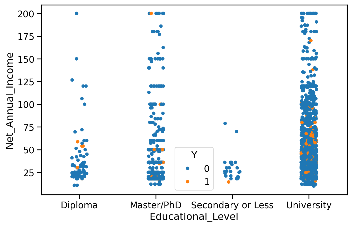
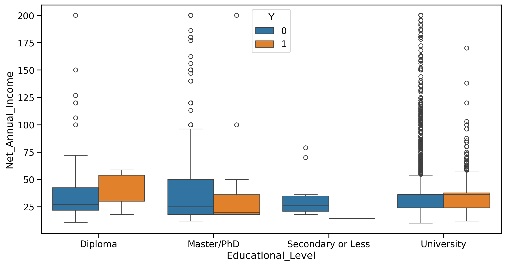
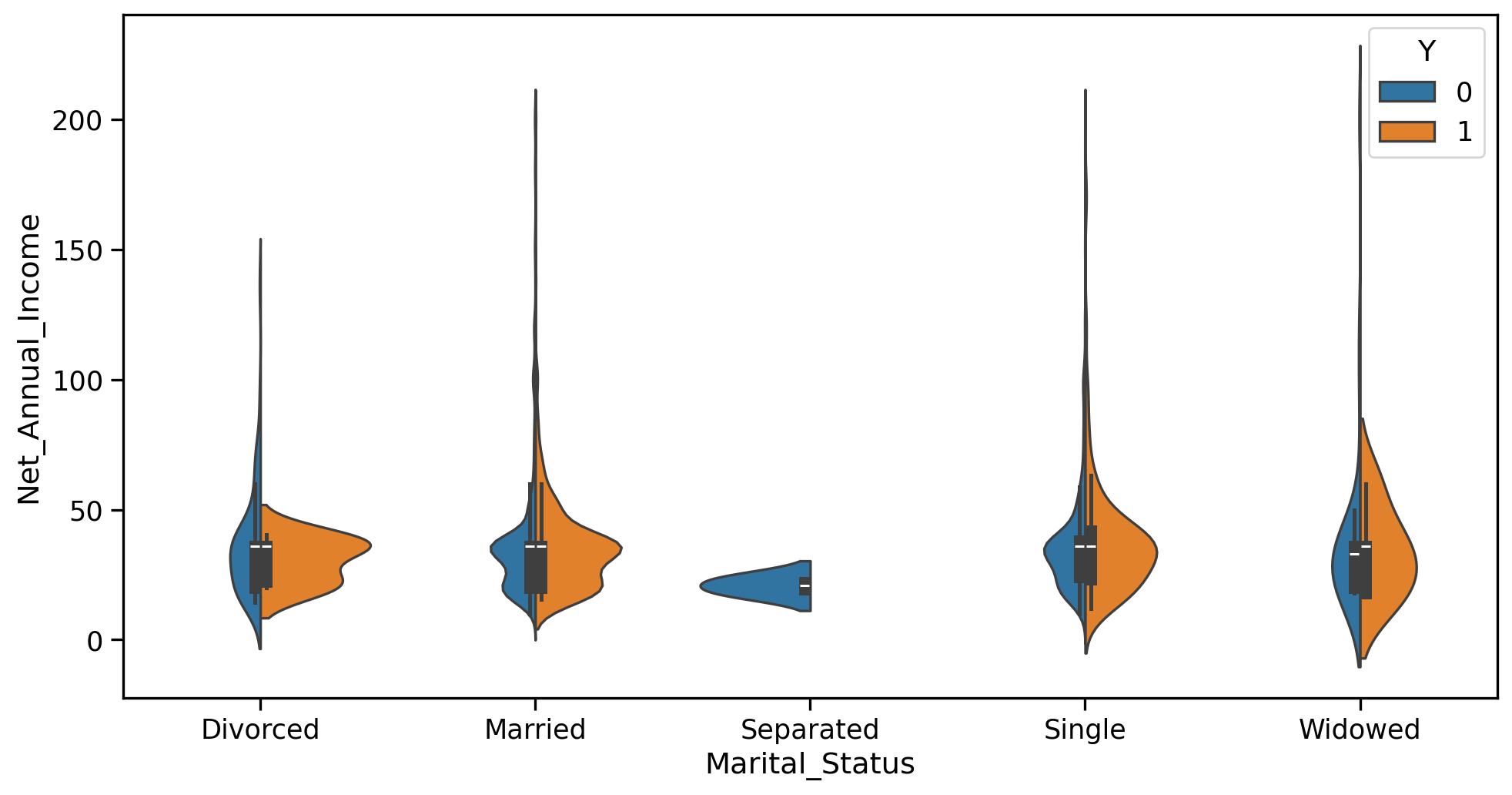
Many of these things can be done right at the beginning, when reading the CSV file, through some options to the pd.read_csv() function. You might need to read carefully its documentation in order to see which options are useful. Once you are happy with your importation and cleaning of the data, you can: - Use pandas and some graphical backend to perform data visualization … - … in order to understand visually the impact of some features on Y (credit was granted or not). For this, you need to decide which plots make sense for this and produce them

We will provide thorough explanations and code that performs all of this in subsequent sessions.

A quick and dirty import

Let’s import the data into a pandas dataframe, as simply as possible The only thing we care about for now is the fact that the column separator is ';' and not ',' (American csv files use , as a default separator, Continental European csv files use ;).

import requests
import os

# The path containing your notebook
path_data = './'
# The name of the file
filename = 'gro.csv.gz'
# the file path
fpath = os.path.join(path_data, filename)

if os.path.exists(fpath):
    print(f'The file "{fpath}" already exists.')
else:
    url = 'https://stephane-v-boucheron.fr/data/gro.csv.gz'
    r = requests.get(url)
    with open(fpath, 'wb') as f:
        f.write(r.content)
    print(f'Downloaded file "{fpath}".')

The file "./gro.csv.gz" already exists.

import numpy as np
import pandas as pd
import plotly.express as px
import matplotlib.pyplot as plt
import seaborn as sns
from pandas import Timestamp
import pickle as pkl

filename = "gro.csv.gz"
df = pd.read_csv(filename, sep=';')
df.head(n=5)

	Id_Customer	Y	Customer_Type	BirthDate	Customer_Open_Date	P_Client	Educational_Level	Marital_Status	Number_Of_Dependant	Years_At_Residence	...	Prod_Sub_Category	Prod_Decision_Date	Source	Type_Of_Residence	Nb_Of_Products	Prod_Closed_Date	Prod_Category	Unnamed: 19	Unnamed: 20	Unnamed: 21
0	6714	0	Non Existing Client	02/09/1971	18/01/2012	NP_Client	University	Married	3.0	10	...	C	23/01/2012	Sales	Owned	1	NaN	B	NaN	NaN	NaN
1	7440	0	Non Existing Client	07/08/1977	13/02/2012	NP_Client	University	Married	3.0	1	...	C	14/02/2012	Sales	Owned	1	NaN	B	NaN	NaN	NaN
2	573	0	Existing Client	13/06/1974	04/02/2009	P_Client	University	Married	0.0	12	...	C	30/06/2011	Sales	Parents	1	NaN	G	NaN	NaN	NaN
3	9194	0	Non Existing Client	07/11/1973	03/04/2012	NP_Client	University	Married	2.0	10	...	C	04/04/2012	Sales	Owned	1	NaN	B	NaN	NaN	NaN
4	3016	1	Existing Client	08/07/1982	25/08/2011	NP_Client	University	Married	3.0	3	...	C	07/09/2011	Sales	New rent	1	31/12/2012	L	NaN	NaN	NaN

5 rows × 22 columns

df.columns

Index(['Id_Customer', 'Y', 'Customer_Type', 'BirthDate', 'Customer_Open_Date',
       'P_Client', 'Educational_Level', 'Marital_Status',
       'Number_Of_Dependant', 'Years_At_Residence', 'Net_Annual_Income',
       'Years_At_Business', 'Prod_Sub_Category', 'Prod_Decision_Date',
       'Source', 'Type_Of_Residence', 'Nb_Of_Products', 'Prod_Closed_Date',
       'Prod_Category', 'Unnamed: 19', 'Unnamed: 20', 'Unnamed: 21'],
      dtype='object')

Remark. There are weird columns at the right end, they look empty. They are not mentioned in the data description (metadata).

df.info()

<class 'pandas.core.frame.DataFrame'>
RangeIndex: 6725 entries, 0 to 6724
Data columns (total 22 columns):
 #   Column               Non-Null Count  Dtype  
---  ------               --------------  -----  
 0   Id_Customer          6725 non-null   int64  
 1   Y                    6725 non-null   int64  
 2   Customer_Type        6725 non-null   object 
 3   BirthDate            6725 non-null   object 
 4   Customer_Open_Date   6725 non-null   object 
 5   P_Client             6725 non-null   object 
 6   Educational_Level    6725 non-null   object 
 7   Marital_Status       6725 non-null   object 
 8   Number_Of_Dependant  6723 non-null   float64
 9   Years_At_Residence   6725 non-null   int64  
 10  Net_Annual_Income    6722 non-null   object 
 11  Years_At_Business    6721 non-null   float64
 12  Prod_Sub_Category    6725 non-null   object 
 13  Prod_Decision_Date   6725 non-null   object 
 14  Source               6725 non-null   object 
 15  Type_Of_Residence    6725 non-null   object 
 16  Nb_Of_Products       6725 non-null   int64  
 17  Prod_Closed_Date     1434 non-null   object 
 18  Prod_Category        6725 non-null   object 
 19  Unnamed: 19          0 non-null      float64
 20  Unnamed: 20          0 non-null      float64
 21  Unnamed: 21          0 non-null      float64
dtypes: float64(5), int64(4), object(13)
memory usage: 1.1+ MB

df["BirthDate"].head()

0    02/09/1971
1    07/08/1977
2    13/06/1974
3    07/11/1973
4    08/07/1982
Name: BirthDate, dtype: object

type(df.loc[0, 'BirthDate'])

str

This means that dates are indeed imported as a strings…

df['Prod_Sub_Category'].head()

0    C
1    C
2    C
3    C
4    C
Name: Prod_Sub_Category, dtype: object

type(df.loc[0, 'Prod_Sub_Category'])

str

Categorical variables are imported as a strings as well

df['Net_Annual_Income'].head(n=10)

0        36
1        36
2        18
3        36
4        36
5    59,916
6        36
7        60
8        36
9        36
Name: Net_Annual_Income, dtype: object

type(df.loc[0, 'Net_Annual_Income'])

str

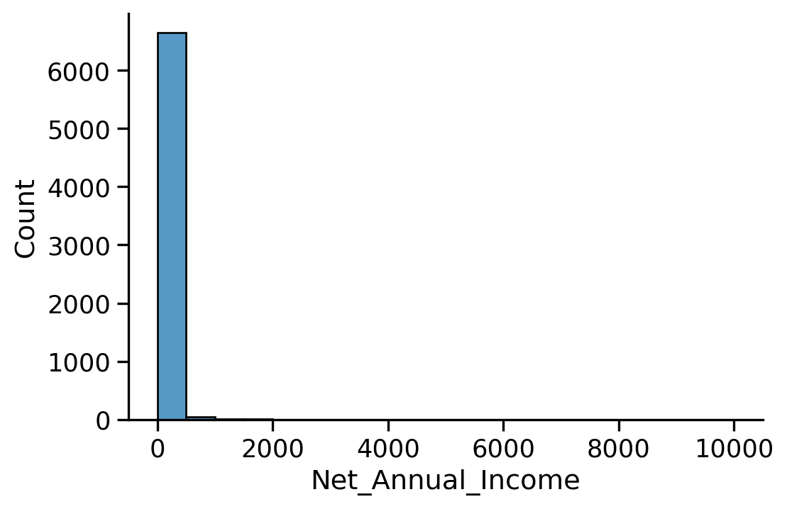
Net actual income is a string as well ! While it is clearly a number !!!

df.describe(include='all')

	Id_Customer	Y	Customer_Type	BirthDate	Customer_Open_Date	P_Client	Educational_Level	Marital_Status	Number_Of_Dependant	Years_At_Residence	...	Prod_Sub_Category	Prod_Decision_Date	Source	Type_Of_Residence	Nb_Of_Products	Prod_Closed_Date	Prod_Category	Unnamed: 19	Unnamed: 20	Unnamed: 21
count	6725.000000	6725.000000	6725	6725	6725	6725	6725	6725	6723.000000	6725.000000	...	6725	6725	6725	6725	6725.000000	1434	6725	0.0	0.0	0.0
unique	NaN	NaN	2	5224	1371	2	4	5	NaN	NaN	...	3	278	2	5	NaN	349	13	NaN	NaN	NaN
top	NaN	NaN	Non Existing Client	01/10/1984	12/12/2011	NP_Client	University	Married	NaN	NaN	...	C	06/12/2011	Sales	Owned	NaN	30/05/2013	B	NaN	NaN	NaN
freq	NaN	NaN	4214	8	50	6213	5981	5268	NaN	NaN	...	5783	58	5149	5986	NaN	116	3979	NaN	NaN	NaN
mean	4821.029740	0.072862	NaN	NaN	NaN	NaN	NaN	NaN	1.051614	12.564758	...	NaN	NaN	NaN	NaN	1.086840	NaN	NaN	NaN	NaN	NaN
std	2775.505395	0.259930	NaN	NaN	NaN	NaN	NaN	NaN	1.332712	9.986257	...	NaN	NaN	NaN	NaN	0.295033	NaN	NaN	NaN	NaN	NaN
min	1.000000	0.000000	NaN	NaN	NaN	NaN	NaN	NaN	0.000000	0.000000	...	NaN	NaN	NaN	NaN	1.000000	NaN	NaN	NaN	NaN	NaN
25%	2399.000000	0.000000	NaN	NaN	NaN	NaN	NaN	NaN	0.000000	4.000000	...	NaN	NaN	NaN	NaN	1.000000	NaN	NaN	NaN	NaN	NaN
50%	4822.000000	0.000000	NaN	NaN	NaN	NaN	NaN	NaN	0.000000	10.000000	...	NaN	NaN	NaN	NaN	1.000000	NaN	NaN	NaN	NaN	NaN
75%	7209.000000	0.000000	NaN	NaN	NaN	NaN	NaN	NaN	2.000000	17.000000	...	NaN	NaN	NaN	NaN	1.000000	NaN	NaN	NaN	NaN	NaN
max	9605.000000	1.000000	NaN	NaN	NaN	NaN	NaN	NaN	20.000000	73.000000	...	NaN	NaN	NaN	NaN	3.000000	NaN	NaN	NaN	NaN	NaN

11 rows × 22 columns

Method describe() delivers a summary for numerical columns. It provides location parameters (mean and median) and scale parameters (standard deviation and Inter Quartile Range (IQR)). For other types of columns it is useless.

df_description = df.describe(include='all')

df_description.index

Index(['count', 'unique', 'top', 'freq', 'mean', 'std', 'min', '25%', '50%',
       '75%', 'max'],
      dtype='object')

Checkup

We have to improve data import.

Here is a list of the problems we face.

The last three columns are empty
Dates are encoded as str (Python string type)
There are many missing values
Categorical features are encoded are str
The Net_Annual_Income is imported as a string

By looking at column names, column descriptions, and common sense, we can infer the type of features we face. There are dates features, numerical features, and categorical features. Some features can be either treated as categorical or numerical.

There are many missing values, that need to be handled.
The annual net income is imported as a string, why?
Dates should be handled as dates and not as strings: this allows us to use the date and time processing functions from the datetime package.

Here is a tentative structure of the features

Numerical features

Years_At_Residence
Net_Annual_Income
Years_At_Business

Features to be decided

Number_Of_Dependant
Nb_Of_Products

Categorical features

Customer_Type
P_Client
Educational_Level
Marital_Status
Prod_Sub_Category
Source
Type_Of_Residence
Prod_Category

Date features

BirthDate
Customer_Open_Date
Prod_Decision_Date
Prod_Closed_Date

A closer look at the import problems

Let us find solutions to all these import problems.

The last three columns are empty

It seems to come from the fact that the data always ends with several ';' characters. We can remove them simply using the usecols option from read_csv.

Passing how=“all” to method dropna() (df.dropna(how="all")) will drop only rows that are all NA:

# all([True, False, True])
# df.isna().map(all)

df.dropna(how="all").info()

<class 'pandas.core.frame.DataFrame'>
RangeIndex: 6725 entries, 0 to 6724
Data columns (total 22 columns):
 #   Column               Non-Null Count  Dtype  
---  ------               --------------  -----  
 0   Id_Customer          6725 non-null   int64  
 1   Y                    6725 non-null   int64  
 2   Customer_Type        6725 non-null   object 
 3   BirthDate            6725 non-null   object 
 4   Customer_Open_Date   6725 non-null   object 
 5   P_Client             6725 non-null   object 
 6   Educational_Level    6725 non-null   object 
 7   Marital_Status       6725 non-null   object 
 8   Number_Of_Dependant  6723 non-null   float64
 9   Years_At_Residence   6725 non-null   int64  
 10  Net_Annual_Income    6722 non-null   object 
 11  Years_At_Business    6721 non-null   float64
 12  Prod_Sub_Category    6725 non-null   object 
 13  Prod_Decision_Date   6725 non-null   object 
 14  Source               6725 non-null   object 
 15  Type_Of_Residence    6725 non-null   object 
 16  Nb_Of_Products       6725 non-null   int64  
 17  Prod_Closed_Date     1434 non-null   object 
 18  Prod_Category        6725 non-null   object 
 19  Unnamed: 19          0 non-null      float64
 20  Unnamed: 20          0 non-null      float64
 21  Unnamed: 21          0 non-null      float64
dtypes: float64(5), int64(4), object(13)
memory usage: 1.1+ MB

Dates are actually `str`

We need to specify which columns must be encoded as dates using the parse_dates option from read_csv. Fortunately enough, pandas is clever enough to interpret the date format.

type(df.loc[0, 'BirthDate'])

str

There is a lot of missing values

We will see below that a single column contains most missing values.

df.isnull().sum()

Id_Customer               0
Y                         0
Customer_Type             0
BirthDate                 0
Customer_Open_Date        0
P_Client                  0
Educational_Level         0
Marital_Status            0
Number_Of_Dependant       2
Years_At_Residence        0
Net_Annual_Income         3
Years_At_Business         4
Prod_Sub_Category         0
Prod_Decision_Date        0
Source                    0
Type_Of_Residence         0
Nb_Of_Products            0
Prod_Closed_Date       5291
Prod_Category             0
Unnamed: 19            6725
Unnamed: 20            6725
Unnamed: 21            6725
dtype: int64

'01/01/1985'

'01/01/1985'

The column Prod_Closed_Date contains mostly missing values !

df[['Prod_Closed_Date']].head(5)

	Prod_Closed_Date
0	NaN
1	NaN
2	NaN
3	NaN
4	31/12/2012

Remove the useless columns and check the remaining missing values

df.drop(['Prod_Closed_Date', 
         'Unnamed: 19', 
         'Unnamed: 20', 
         'Unnamed: 21'], 
         axis="columns", 
         inplace=True)

df.head()

	Id_Customer	Y	Customer_Type	BirthDate	Customer_Open_Date	P_Client	Educational_Level	Marital_Status	Number_Of_Dependant	Years_At_Residence	Net_Annual_Income	Years_At_Business	Prod_Sub_Category	Prod_Decision_Date	Source	Type_Of_Residence	Nb_Of_Products	Prod_Category
0	6714	0	Non Existing Client	02/09/1971	18/01/2012	NP_Client	University	Married	3.0	10	36	3.0	C	23/01/2012	Sales	Owned	1	B
1	7440	0	Non Existing Client	07/08/1977	13/02/2012	NP_Client	University	Married	3.0	1	36	1.0	C	14/02/2012	Sales	Owned	1	B
2	573	0	Existing Client	13/06/1974	04/02/2009	P_Client	University	Married	0.0	12	18	2.0	C	30/06/2011	Sales	Parents	1	G
3	9194	0	Non Existing Client	07/11/1973	03/04/2012	NP_Client	University	Married	2.0	10	36	1.0	C	04/04/2012	Sales	Owned	1	B
4	3016	1	Existing Client	08/07/1982	25/08/2011	NP_Client	University	Married	3.0	3	36	1.0	C	07/09/2011	Sales	New rent	1	L

Let’s display the rows with missing values and let’s highlight them

df[df.isnull().any(axis="columns")]\
  .style\
  .highlight_null()

	Id_Customer	Y	Customer_Type	BirthDate	Customer_Open_Date	P_Client	Educational_Level	Marital_Status	Number_Of_Dependant	Years_At_Residence	Net_Annual_Income	Years_At_Business	Prod_Sub_Category	Prod_Decision_Date	Source	Type_Of_Residence	Nb_Of_Products	Prod_Category
105	9407	0	Non Existing Client	17/05/1956	17/04/2012	NP_Client	University	Married	0.000000	1	36	nan	C	18/04/2012	Sales	Owned	1	D
793	8953	1	Existing Client	07/06/1990	20/09/2010	P_Client	University	Single	nan	21	33,6	1.000000	C	18/04/2012	Branch	Owned	2	G
2349	9399	0	Non Existing Client	16/04/1968	17/04/2012	NP_Client	University	Married	0.000000	10	nan	10.000000	C	18/04/2012	Sales	Owned	1	B
2400	8826	0	Existing Client	03/01/1980	20/03/2005	NP_Client	University	Married	1.000000	8	nan	9.000000	C	17/04/2012	Branch	Owned	1	B
2484	398	0	Non Existing Client	14/05/1984	19/05/2011	NP_Client	Master/PhD	Single	0.000000	10	25	nan	C	26/05/2011	Branch	Owned	2	D
3438	5882	0	Non Existing Client	08/08/1981	14/12/2011	NP_Client	University	Married	0.000000	2	108	nan	C	27/12/2011	Branch	Owned	1	B
6307	9588	0	Existing Client	05/07/1950	18/09/2004	NP_Client	Master/PhD	Married	nan	10	50	10.000000	C	26/04/2012	Sales	Owned	1	B
6355	8777	0	Existing Client	10/09/1985	18/09/2003	NP_Client	Master/PhD	Single	0.000000	26	36	nan	C	19/03/2012	Branch	Owned	1	D
6431	9555	0	Non Existing Client	15/01/1951	23/04/2012	NP_Client	University	Married	0.000000	11	nan	0.000000	C	26/04/2012	Branch	Old rent	2	B

Categorial features are `str`

We need to say the dtype we want to use for some columns using the dtype option of read_csv.

type(df.loc[0, 'Prod_Sub_Category'])

str

df['Prod_Sub_Category'].unique()

array(['C', 'G', 'P'], dtype=object)

The annual net income is imported as a string

This problem comes from the fact that the decimal separator is in continental European notation: it’s a ',' and not a '.', so we need to specify it using the decimal option to read_csv.

type(df.loc[0, 'Net_Annual_Income'])

str

df['Net_Annual_Income'].head(n=10)

0        36
1        36
2        18
3        36
4        36
5    59,916
6        36
7        60
8        36
9        36
Name: Net_Annual_Income, dtype: object

A better import of the data

We build a dict that specifies the dtype to use for each column and pass it to read_csv() using the dtype option
We also specify the decimal, usecols and parse_dates options

Note

Some columns could be imported as int.

However, pandas is built above numpy, pandas does not support columns with integer dtype and missing values.

As columnn type inference does not work universally, a safeguard consists in providing read_csv() with optinal argument dtype. The default value is None. The default value is overriden by a dictionary where keys are strings denoting the column names where type inference is not satisfactory and values denote the desired types.

gro_dtypes = {
    'Years_At_Residence': np.int64,
    'Net_Annual_Income' : np.float64,
    'Years_At_Business': np.float64,
    'Number_Of_Dependant': np.float64,
    'Nb_Of_Products': np.int64,
    'Customer_Type': 'category',
    'P_Client': 'category',
    'Educational_Level': 'category',
    'Marital_Status': 'category',
    'Prod_Sub_Category': 'category',
    'Source': 'category',
    'Type_Of_Residence': 'category',
    'Prod_Category': 'category',
}

Note

Note that the intended type is 'category', the function still has to infer the categories from the data, and to build the actual categorical type with a proper encoding.

We can use the dictionary unpacking capabilities of Python to save the overriden keyword parameters into a dictionary. The dictionary can be serialized and saved on disc. It is then considered as metadat.

gro_read_spec_dict = {
    'sep': ';',      # continental separator
    'decimal': ',',  # continental decimal separator
    'usecols': range(19),  # Range of the columns to keep (remove the last three ones)
    'parse_dates': ['BirthDate', # Which columns should be parsed as dates ?
                    'Customer_Open_Date', 
                    'Prod_Decision_Date', 
                    'Prod_Closed_Date'],
    'dtype': gro_dtypes  # Specify some dtypes
  }

Using the metadata packed into the dictionary turns easy and concise. The same metadata can be reused for any csv file with the same features.

df = pd.read_csv(
    "gro.csv.gz",      # Filename
    ** gro_read_spec_dict
)

/tmp/ipykernel_14457/1983308737.py:1: UserWarning:

Parsing dates in %d/%m/%Y format when dayfirst=False (the default) was specified. Pass `dayfirst=True` or specify a format to silence this warning.

/tmp/ipykernel_14457/1983308737.py:1: UserWarning:

Parsing dates in %d/%m/%Y format when dayfirst=False (the default) was specified. Pass `dayfirst=True` or specify a format to silence this warning.

/tmp/ipykernel_14457/1983308737.py:1: UserWarning:

Parsing dates in %d/%m/%Y format when dayfirst=False (the default) was specified. Pass `dayfirst=True` or specify a format to silence this warning.

df.info()

<class 'pandas.core.frame.DataFrame'>
RangeIndex: 6725 entries, 0 to 6724
Data columns (total 19 columns):
 #   Column               Non-Null Count  Dtype         
---  ------               --------------  -----         
 0   Id_Customer          6725 non-null   int64         
 1   Y                    6725 non-null   int64         
 2   Customer_Type        6725 non-null   category      
 3   BirthDate            6725 non-null   object        
 4   Customer_Open_Date   6725 non-null   datetime64[ns]
 5   P_Client             6725 non-null   category      
 6   Educational_Level    6725 non-null   category      
 7   Marital_Status       6725 non-null   category      
 8   Number_Of_Dependant  6723 non-null   float64       
 9   Years_At_Residence   6725 non-null   int64         
 10  Net_Annual_Income    6722 non-null   float64       
 11  Years_At_Business    6721 non-null   float64       
 12  Prod_Sub_Category    6725 non-null   category      
 13  Prod_Decision_Date   6725 non-null   datetime64[ns]
 14  Source               6725 non-null   category      
 15  Type_Of_Residence    6725 non-null   category      
 16  Nb_Of_Products       6725 non-null   int64         
 17  Prod_Closed_Date     1434 non-null   datetime64[ns]
 18  Prod_Category        6725 non-null   category      
dtypes: category(8), datetime64[ns](3), float64(3), int64(4), object(1)
memory usage: 632.1+ KB

Note

Column BirthDate is meant to be a date column. Nevertheless, is is not converted to a date or datetime column.

If a column or index cannot be represented as an array of datetime, say because of an unparsable value or a mixture of timezones, the column or index will be returned unaltered as an object data type. For non-standard datetime parsing, use to_datetime() after read_csv().

If we do not set optional arguments, pd.to_datetime() fails to convert df['BirthDate'].

bd = pd.to_datetime(df['BirthDate'])

We get a message:

ValueError: time data “13/06/1974” doesn’t match format “%m/%d/%Y”, at position 2. You might want to try: - passing format if your strings have a consistent format; - passing format='ISO8601' if your strings are all ISO8601 but not necessarily in exactly the same format; - passing format='mixed', and the format will be inferred for each element individually. You might want to use dayfirst alongside this.

Indeed, the format of the first items in column BirthDate seems to be %d/%m/%Y (as for the other date columns).

An easy fix consists in setting optional argument dayfirst to True.

egg = pd.to_datetime(df['BirthDate'], dayfirst=True)

A possibly safer

spam = pd.to_datetime(df['BirthDate'], format='%d/%m/%Y')

np.all(spam==egg)

True

We can improve our import by enriching our dictionary of optional arguments.

gro_read_spec_dict['date_format']= '%d/%m/%Y'

df = pd.read_csv(
    "gro.csv.gz",      # Filename
    ** gro_read_spec_dict
)

df.info()

<class 'pandas.core.frame.DataFrame'>
RangeIndex: 6725 entries, 0 to 6724
Data columns (total 19 columns):
 #   Column               Non-Null Count  Dtype         
---  ------               --------------  -----         
 0   Id_Customer          6725 non-null   int64         
 1   Y                    6725 non-null   int64         
 2   Customer_Type        6725 non-null   category      
 3   BirthDate            6725 non-null   datetime64[ns]
 4   Customer_Open_Date   6725 non-null   datetime64[ns]
 5   P_Client             6725 non-null   category      
 6   Educational_Level    6725 non-null   category      
 7   Marital_Status       6725 non-null   category      
 8   Number_Of_Dependant  6723 non-null   float64       
 9   Years_At_Residence   6725 non-null   int64         
 10  Net_Annual_Income    6722 non-null   float64       
 11  Years_At_Business    6721 non-null   float64       
 12  Prod_Sub_Category    6725 non-null   category      
 13  Prod_Decision_Date   6725 non-null   datetime64[ns]
 14  Source               6725 non-null   category      
 15  Type_Of_Residence    6725 non-null   category      
 16  Nb_Of_Products       6725 non-null   int64         
 17  Prod_Closed_Date     1434 non-null   datetime64[ns]
 18  Prod_Category        6725 non-null   category      
dtypes: category(8), datetime64[ns](4), float64(3), int64(4)
memory usage: 632.1 KB

df['Prod_Sub_Category'].head()

0    C
1    C
2    C
3    C
4    C
Name: Prod_Sub_Category, dtype: category
Categories (3, object): ['C', 'G', 'P']

type(df.loc[0, 'BirthDate'])

pandas._libs.tslibs.timestamps.Timestamp

Let us remove Prod_Closed_Date (mostly contains missing values)

prod_closed_date = df.pop('Prod_Closed_Date')
df.shape

(6725, 18)

df.info()

<class 'pandas.core.frame.DataFrame'>
RangeIndex: 6725 entries, 0 to 6724
Data columns (total 18 columns):
 #   Column               Non-Null Count  Dtype         
---  ------               --------------  -----         
 0   Id_Customer          6725 non-null   int64         
 1   Y                    6725 non-null   int64         
 2   Customer_Type        6725 non-null   category      
 3   BirthDate            6725 non-null   datetime64[ns]
 4   Customer_Open_Date   6725 non-null   datetime64[ns]
 5   P_Client             6725 non-null   category      
 6   Educational_Level    6725 non-null   category      
 7   Marital_Status       6725 non-null   category      
 8   Number_Of_Dependant  6723 non-null   float64       
 9   Years_At_Residence   6725 non-null   int64         
 10  Net_Annual_Income    6722 non-null   float64       
 11  Years_At_Business    6721 non-null   float64       
 12  Prod_Sub_Category    6725 non-null   category      
 13  Prod_Decision_Date   6725 non-null   datetime64[ns]
 14  Source               6725 non-null   category      
 15  Type_Of_Residence    6725 non-null   category      
 16  Nb_Of_Products       6725 non-null   int64         
 17  Prod_Category        6725 non-null   category      
dtypes: category(8), datetime64[ns](3), float64(3), int64(4)
memory usage: 579.6 KB

And remove the remaining rows with missing values

print(df.shape)
df = df.dropna()
print(df.shape)

(6725, 18)
(6716, 18)

# Now we save the cleaned dataset into a CSV file
df.to_csv("gro_cleaned.csv")

!ls -al gro_*

-rw-rw-r-- 1 boucheron boucheron 849755 févr.  5 21:59 gro_cleaned.csv
-rw-rw-r-- 1 boucheron boucheron 282610 févr.  5 19:20 gro_cleaned.feather
-rw-rw-r-- 1 boucheron boucheron 211956 févr.  5 19:20 gro_cleaned.parquet
-rw-rw-r-- 1 boucheron boucheron 647772 févr.  5 19:20 gro_cleaned.pkl
-rw-rw-r-- 1 boucheron boucheron 753398 févr.  5 19:20 gro_training.pkl

Note

Read the Data loading section in the Pandas book

We used the following subsections:

Type inference and data conversion
Date and time parsing
Unclean data issues

pandas.read_csv() has around 50 optional/keywords parameters.

cleaned_spec_dict = {
    'parse_dates': ['BirthDate', 
                    'Customer_Open_Date', 
                    'Prod_Decision_Date'],
    'dtype': gro_dtypes  
}

df = pd.read_csv("gro_cleaned.csv", 
    **cleaned_spec_dict)

df.info()

<class 'pandas.core.frame.DataFrame'>
RangeIndex: 6716 entries, 0 to 6715
Data columns (total 19 columns):
 #   Column               Non-Null Count  Dtype         
---  ------               --------------  -----         
 0   Unnamed: 0           6716 non-null   int64         
 1   Id_Customer          6716 non-null   int64         
 2   Y                    6716 non-null   int64         
 3   Customer_Type        6716 non-null   category      
 4   BirthDate            6716 non-null   datetime64[ns]
 5   Customer_Open_Date   6716 non-null   datetime64[ns]
 6   P_Client             6716 non-null   category      
 7   Educational_Level    6716 non-null   category      
 8   Marital_Status       6716 non-null   category      
 9   Number_Of_Dependant  6716 non-null   float64       
 10  Years_At_Residence   6716 non-null   int64         
 11  Net_Annual_Income    6716 non-null   float64       
 12  Years_At_Business    6716 non-null   float64       
 13  Prod_Sub_Category    6716 non-null   category      
 14  Prod_Decision_Date   6716 non-null   datetime64[ns]
 15  Source               6716 non-null   category      
 16  Type_Of_Residence    6716 non-null   category      
 17  Nb_Of_Products       6716 non-null   int64         
 18  Prod_Category        6716 non-null   category      
dtypes: category(8), datetime64[ns](3), float64(3), int64(5)
memory usage: 631.3 KB

Comment on file formats

You can use other methods starting with .to_XX to save in another format.

OK to use csv for “small” datasets (several MB). But this is not a self-documented format.
Use pickle for more compressed and faster format (limited to 4GB). It’s the standard binary serialization format of Python
feather is another fast and lightweight file format for storing data frames. A very popular exchange format.
parquet is a format for big distributed data (works nicely with Spark)

among several others…

Note

Have a look at the PyArrow package

df.index

RangeIndex(start=0, stop=6716, step=1)

df.to_pickle("gro_cleaned.pkl")
df.to_parquet("gro_cleaned.parquet")
df.reset_index().to_feather("gro_cleaned.feather")

df.index

RangeIndex(start=0, stop=6716, step=1)

And you can read again using the corresponding read_XX function

df = pd.read_pickle("gro_cleaned.pkl")
df.info()

<class 'pandas.core.frame.DataFrame'>
RangeIndex: 6716 entries, 0 to 6715
Data columns (total 19 columns):
 #   Column               Non-Null Count  Dtype         
---  ------               --------------  -----         
 0   Unnamed: 0           6716 non-null   int64         
 1   Id_Customer          6716 non-null   int64         
 2   Y                    6716 non-null   int64         
 3   Customer_Type        6716 non-null   category      
 4   BirthDate            6716 non-null   datetime64[ns]
 5   Customer_Open_Date   6716 non-null   datetime64[ns]
 6   P_Client             6716 non-null   category      
 7   Educational_Level    6716 non-null   category      
 8   Marital_Status       6716 non-null   category      
 9   Number_Of_Dependant  6716 non-null   float64       
 10  Years_At_Residence   6716 non-null   int64         
 11  Net_Annual_Income    6716 non-null   float64       
 12  Years_At_Business    6716 non-null   float64       
 13  Prod_Sub_Category    6716 non-null   category      
 14  Prod_Decision_Date   6716 non-null   datetime64[ns]
 15  Source               6716 non-null   category      
 16  Type_Of_Residence    6716 non-null   category      
 17  Nb_Of_Products       6716 non-null   int64         
 18  Prod_Category        6716 non-null   category      
dtypes: category(8), datetime64[ns](3), float64(3), int64(5)
memory usage: 630.0 KB

!ls -alh gro_cleaned*

-rw-rw-r-- 1 boucheron boucheron 830K févr.  5 21:59 gro_cleaned.csv
-rw-rw-r-- 1 boucheron boucheron 276K févr.  5 21:59 gro_cleaned.feather
-rw-rw-r-- 1 boucheron boucheron 207K févr.  5 21:59 gro_cleaned.parquet
-rw-rw-r-- 1 boucheron boucheron 633K févr.  5 21:59 gro_cleaned.pkl

The net income columns is very weird

income = df['Net_Annual_Income']
income.describe()

count     6716.000000
mean        60.954422
std        235.973454
min          0.001000
25%         20.000000
50%         36.000000
75%         36.000000
max      10000.000000
Name: Net_Annual_Income, dtype: float64

(income <= 100).sum(), (income > 100).sum()

(6281, 435)

Most values are smaller than 100, while some are much much larger…

%matplotlib inline

sns.set_context("notebook", font_scale=1.2)

sns.displot(x='Net_Annual_Income', 
            data=df, 
            bins=20,
            height=4, 
            aspect=1.5)

This is annoying, we don’t really see much…

sns.displot(x='Net_Annual_Income', 
            data=df, 
            bins=20, 
            height=4, 
            aspect=1.5, 
            log_scale=(False, True))

Distribution for less than 100K revenue

sns.displot(x='Net_Annual_Income', 
            data=df[df['Net_Annual_Income'] < 100], 
            bins=15, 
            height=4, 
            aspect=1.5)

Distribution for less than 400K revenue

sns.displot(x='Net_Annual_Income',
            data=df[df['Net_Annual_Income'] < 400], 
            bins=15, 
            height=4, 
            aspect=1.5)

(df['Net_Annual_Income'] == 36.0).sum()

income_counts = (
    pd.DataFrame({
        "income_category": df['Net_Annual_Income'].astype("category"),
        "income": df['Net_Annual_Income']
    })
    .groupby("income_category")
    .count()
    .reset_index()
    .rename(columns={"income": "#customers"})
    .sort_values(by="#customers", 
                 axis="index", 
                 ascending=False)
)

income_counts["%cummulative clients"] \
    = income_counts["#customers"].cumsum() / income_counts["#customers"].sum()

( 
    income_counts
        .iloc[:20]
        .style.bar(subset=["%cummulative clients"],         vmin=0, vmax=1)
)

/tmp/ipykernel_14457/1697804417.py:6: FutureWarning:

The default of observed=False is deprecated and will be changed to True in a future version of pandas. Pass observed=False to retain current behavior or observed=True to adopt the future default and silence this warning.

	income_category	#customers	%cummulative clients
228	36.000000	2265	0.337254
31	18.000000	1087	0.499107
43	20.000000	538	0.579214
156	30.000000	506	0.654556
318	50.000000	317	0.701757
98	25.000000	314	0.748511
481	100.000000	109	0.764741
84	24.000000	101	0.779780
370	60.000000	95	0.793925
518	120.000000	57	0.802412
267	42.000000	44	0.808964
416	72.000000	40	0.814920
309	48.000000	36	0.820280
562	200.000000	29	0.824598
253	40.000000	25	0.828320
440	80.000000	25	0.832043
536	150.000000	23	0.835468
20	12.000000	22	0.838743
573	250.000000	22	0.842019
598	500.000000	21	0.845146

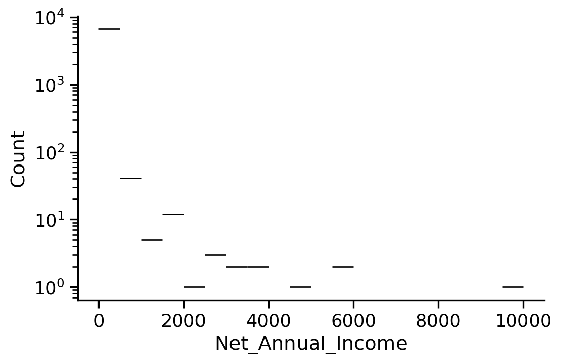
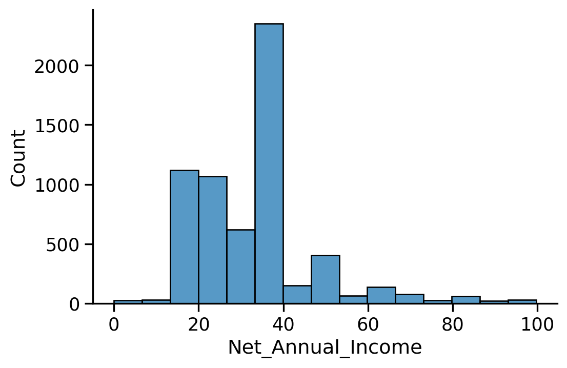
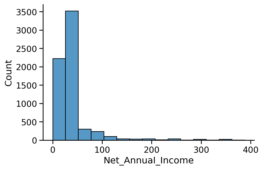
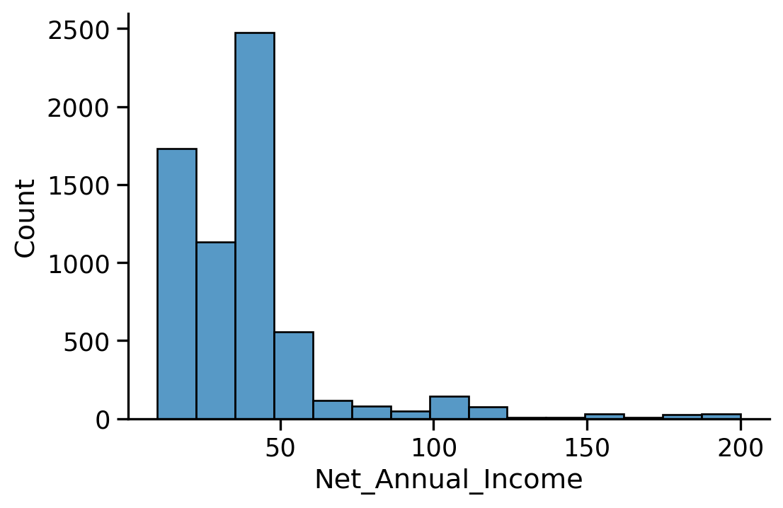
We have some overrepresented values (many possible explanations for this)
To clean the data, we can, for instance, keep only the revenues between [10, 200], or leave it as such

df = df[(df['Net_Annual_Income'] >= 10) & (df['Net_Annual_Income'] <= 200)]

sns.displot(x='Net_Annual_Income', data=df, bins=15, height=4, aspect=1.5)

Some data visualization with `pandas` + `seaborn`

plt.figure(figsize=(8, 5))

sns.stripplot(x='Educational_Level', 
              y='Net_Annual_Income', 
              hue='Y', 
              jitter=True, 
              data=df)

plt.figure(figsize=(12, 6))
sns.boxplot(x='Educational_Level', y='Net_Annual_Income', 
            hue='Y', data=df)

plt.figure(figsize=(12, 6))

sns.violinplot(x='Marital_Status', y='Net_Annual_Income', 
               hue='Y', split=True, data=df)

plt.figure(figsize=(10, 5))

sns.countplot(x='Marital_Status', hue='Y', data=df)

fig, axes = plt.subplots(nrows=4, ncols=3, figsize=(16, 16))

columns = ['Customer_Type', 'P_Client', 'Educational_Level', 
           'Number_Of_Dependant', 'Marital_Status', 'Prod_Sub_Category',
           'Source', 'Type_Of_Residence', 'Nb_Of_Products', 
           'Prod_Category', 'Y']

for i, colname in enumerate(columns):
    sns.countplot(x=colname, data=df, ax=fig.axes[i])


plt.tight_layout()

Final preparation of the dataset

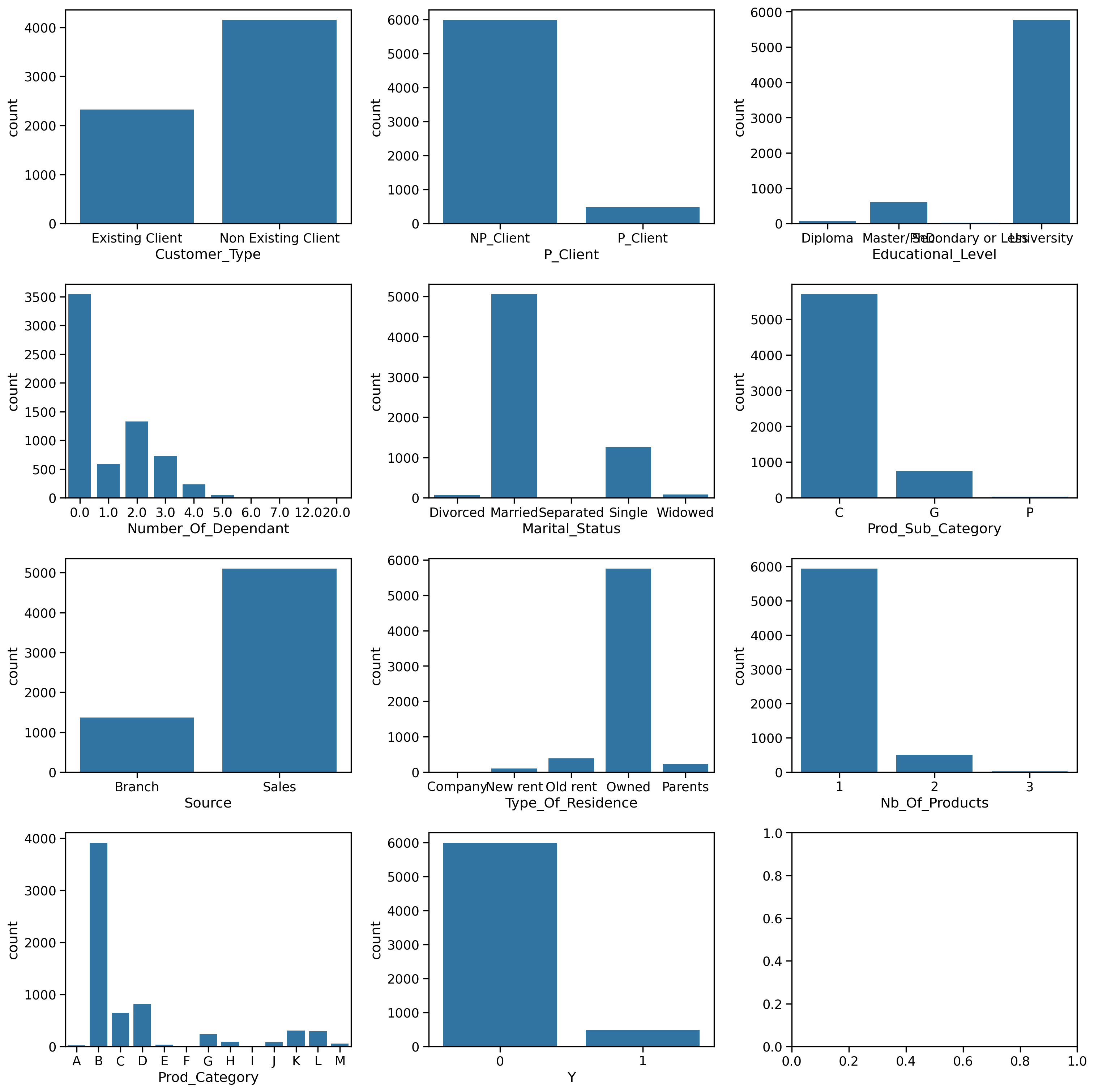
# First we make lists of continuous, categorial and date features

cnt_featnames = [
    'Years_At_Residence',
    'Net_Annual_Income',
    'Years_At_Business',
    'Number_Of_Dependant'
]

cat_featnames = [
    'Customer_Type',
    'P_Client',
    'Educational_Level',
    'Marital_Status',
    'Prod_Sub_Category',
    'Source',
    'Type_Of_Residence',
    'Prod_Category',
    'Nb_Of_Products'
]

date_featnames = [
    'BirthDate',
    'Customer_Open_Date',
    'Prod_Decision_Date'
    #'Prod_Closed_Date'
]

Creation of the features matrix

df[cnt_featnames].head()

	Years_At_Residence	Net_Annual_Income	Years_At_Business	Number_Of_Dependant
0	10	36.0	3.0	3.0
1	1	36.0	1.0	3.0
2	12	18.0	2.0	0.0
3	10	36.0	1.0	2.0
4	3	36.0	1.0	3.0

bin_features = pd.get_dummies(df[cat_featnames],
                              prefix_sep='#', 
                              drop_first=True)

bin_features.head()

	Nb_Of_Products	Customer_Type#Non Existing Client	P_Client#P_Client	Educational_Level#Master/PhD	Educational_Level#Secondary or Less	Educational_Level#University	Marital_Status#Married	Marital_Status#Separated	Marital_Status#Single	Marital_Status#Widowed	...	Prod_Category#D	Prod_Category#E	Prod_Category#F	Prod_Category#G	Prod_Category#H	Prod_Category#I	Prod_Category#J	Prod_Category#K	Prod_Category#L	Prod_Category#M
0	1	True	False	False	False	True	True	False	False	False	...	False	False	False	False	False	False	False	False	False	False
1	1	True	False	False	False	True	True	False	False	False	...	False	False	False	False	False	False	False	False	False	False
2	1	False	True	False	False	True	True	False	False	False	...	False	False	False	True	False	False	False	False	False	False
3	1	True	False	False	False	True	True	False	False	False	...	False	False	False	False	False	False	False	False	False	False
4	1	False	False	False	False	True	True	False	False	False	...	False	False	False	False	False	False	False	False	True	False

5 rows × 29 columns

cnt_features = df[cnt_featnames]
cnt_features.head()

	Years_At_Residence	Net_Annual_Income	Years_At_Business	Number_Of_Dependant
0	10	36.0	3.0	3.0
1	1	36.0	1.0	3.0
2	12	18.0	2.0	0.0
3	10	36.0	1.0	2.0
4	3	36.0	1.0	3.0

def age(x):
    today = Timestamp.today()
    return (today - x).dt.days

date_features = df[date_featnames].apply(age, axis="index")

date_features.head()

	BirthDate	Customer_Open_Date	Prod_Decision_Date
0	19149	4401	4396
1	16983	4375	4374
2	18134	5479	4603
3	18352	4325	4324
4	15187	4547	4534

today = Timestamp.today()
today

Timestamp('2024-02-05 21:59:10.660791')

tt = (today - df["BirthDate"]).loc[0]

(today - df["BirthDate"]).dt.days

0       19149
1       16983
2       18134
3       18352
4       15187
        ...  
6711    25953
6712    15229
6713    26772
6714    14798
6715    15231
Name: BirthDate, Length: 6473, dtype: int64

tt

Timedelta('19149 days 21:59:10.660791')

Final features matrix

all_features = pd.concat([bin_features, cnt_features, date_features], axis=1)

all_features.columns

Index(['Nb_Of_Products', 'Customer_Type#Non Existing Client',
       'P_Client#P_Client', 'Educational_Level#Master/PhD',
       'Educational_Level#Secondary or Less', 'Educational_Level#University',
       'Marital_Status#Married', 'Marital_Status#Separated',
       'Marital_Status#Single', 'Marital_Status#Widowed',
       'Prod_Sub_Category#G', 'Prod_Sub_Category#P', 'Source#Sales',
       'Type_Of_Residence#New rent', 'Type_Of_Residence#Old rent',
       'Type_Of_Residence#Owned', 'Type_Of_Residence#Parents',
       'Prod_Category#B', 'Prod_Category#C', 'Prod_Category#D',
       'Prod_Category#E', 'Prod_Category#F', 'Prod_Category#G',
       'Prod_Category#H', 'Prod_Category#I', 'Prod_Category#J',
       'Prod_Category#K', 'Prod_Category#L', 'Prod_Category#M',
       'Years_At_Residence', 'Net_Annual_Income', 'Years_At_Business',
       'Number_Of_Dependant', 'BirthDate', 'Customer_Open_Date',
       'Prod_Decision_Date'],
      dtype='object')

all_features.head()

	Nb_Of_Products	Customer_Type#Non Existing Client	P_Client#P_Client	Educational_Level#Master/PhD	Educational_Level#Secondary or Less	Educational_Level#University	Marital_Status#Married	Marital_Status#Separated	Marital_Status#Single	Marital_Status#Widowed	...	Prod_Category#K	Prod_Category#L	Prod_Category#M	Years_At_Residence	Net_Annual_Income	Years_At_Business	Number_Of_Dependant	BirthDate	Customer_Open_Date	Prod_Decision_Date
0	1	True	False	False	False	True	True	False	False	False	...	False	False	False	10	36.0	3.0	3.0	19149	4401	4396
1	1	True	False	False	False	True	True	False	False	False	...	False	False	False	1	36.0	1.0	3.0	16983	4375	4374
2	1	False	True	False	False	True	True	False	False	False	...	False	False	False	12	18.0	2.0	0.0	18134	5479	4603
3	1	True	False	False	False	True	True	False	False	False	...	False	False	False	10	36.0	1.0	2.0	18352	4325	4324
4	1	False	False	False	False	True	True	False	False	False	...	False	True	False	3	36.0	1.0	3.0	15187	4547	4534

5 rows × 36 columns

df_debile = pd.DataFrame({"nom etudiant": ["yiyang", "jaouad", "mokhtar", "massil", "simon"], 
              "portable": [True, True, None, True, False]})

df_debile

	nom etudiant	portable
0	yiyang	True
1	jaouad	True
2	mokhtar	None
3	massil	True
4	simon	False

df_debile.index

RangeIndex(start=0, stop=5, step=1)

df_debile.dropna().index

Index([0, 1, 3, 4], dtype='int64')

df_debile.info()

<class 'pandas.core.frame.DataFrame'>
RangeIndex: 5 entries, 0 to 4
Data columns (total 2 columns):
 #   Column        Non-Null Count  Dtype 
---  ------        --------------  ----- 
 0   nom etudiant  5 non-null      object
 1   portable      4 non-null      object
dtypes: object(2)
memory usage: 208.0+ bytes

Note

We removed rows that contained missing values. The index of the dataframe is therefore not contiguous anymore

all_features.index.max()

This could be a problem for later. So let’s reset the index to get a contiguous one

all_features.shape

(6473, 36)

all_features.reset_index(inplace=True, drop=True)

Note

Why does the index matter?

For example, when adding a new column to a dataframe, only items from the new series that have a corresponding index in the Dataframe will be added. The receiving dataframe is not extended to accomodate the new series.

all_features.head()

	Nb_Of_Products	Customer_Type#Non Existing Client	P_Client#P_Client	Educational_Level#Master/PhD	Educational_Level#Secondary or Less	Educational_Level#University	Marital_Status#Married	Marital_Status#Separated	Marital_Status#Single	Marital_Status#Widowed	...	Prod_Category#K	Prod_Category#L	Prod_Category#M	Years_At_Residence	Net_Annual_Income	Years_At_Business	Number_Of_Dependant	BirthDate	Customer_Open_Date	Prod_Decision_Date
0	1	True	False	False	False	True	True	False	False	False	...	False	False	False	10	36.0	3.0	3.0	19149	4401	4396
1	1	True	False	False	False	True	True	False	False	False	...	False	False	False	1	36.0	1.0	3.0	16983	4375	4374
2	1	False	True	False	False	True	True	False	False	False	...	False	False	False	12	18.0	2.0	0.0	18134	5479	4603
3	1	True	False	False	False	True	True	False	False	False	...	False	False	False	10	36.0	1.0	2.0	18352	4325	4324
4	1	False	False	False	False	True	True	False	False	False	...	False	True	False	3	36.0	1.0	3.0	15187	4547	4534

5 rows × 36 columns

Let’s save the data using `pickle`

X = all_features
y = df['Y']

# Let's put eveything in a dictionary
df_pkl = {}
# The features and the labels
df_pkl['features'] = X
df_pkl['labels'] = y
# And also the list of columns we built above
df_pkl['cnt_featnames'] = cnt_featnames
df_pkl['cat_featnames'] = cat_featnames
df_pkl['date_featnames'] = date_featnames

with open("gro_training.pkl", 'wb') as f:
    pkl.dump(df_pkl, f)

!ls -al gro*

-rw-rw-r-- 1 boucheron boucheron 849755 févr.  5 21:59 gro_cleaned.csv
-rw-rw-r-- 1 boucheron boucheron 282610 févr.  5 21:59 gro_cleaned.feather
-rw-rw-r-- 1 boucheron boucheron 211956 févr.  5 21:59 gro_cleaned.parquet
-rw-rw-r-- 1 boucheron boucheron 647772 févr.  5 21:59 gro_cleaned.pkl
-rw-rw-r-- 1 boucheron boucheron 827247 févr.  2 10:38 gro.csv
-rw-rw-r-- 1 boucheron boucheron 134453 févr.  5 16:12 gro.csv.gz
-rw-rw-r-- 1 boucheron boucheron 753398 févr.  5 21:59 gro_training.pkl

The preprocessed data is saved in a pickle file called gro_training.pkl.

Misc: Graphics with `plotly`

Pandas Plotly backend

Plotly express box

fig = px.box(df, 
             x='Marital_Status', 
             y='Net_Annual_Income',
             color='Y')

fig.show()

/home/boucheron/.local/lib/python3.10/site-packages/plotly/express/_core.py:2065: FutureWarning:

When grouping with a length-1 list-like, you will need to pass a length-1 tuple to get_group in a future version of pandas. Pass `(name,)` instead of `name` to silence this warning.

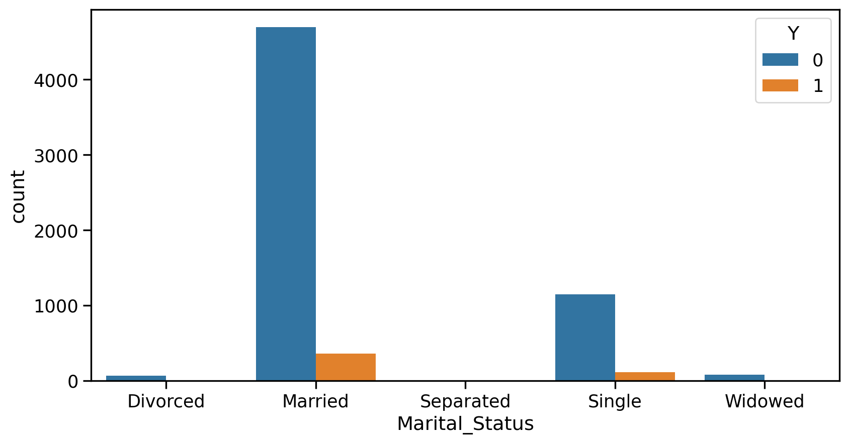
s = df['Marital_Status'].value_counts()

df_counts = pd.DataFrame({
    'status': s.index.to_list(),
    'count': s.to_list()}
)

fig = px.bar(df_counts, 
    x="status", 
    y="count", 
    title="Marital Status")

fig.show()

Your job

A quick and dirty import

Checkup

A closer look at the import problems

The last three columns are empty

Dates are actually str

There is a lot of missing values

Categorial features are str

The annual net income is imported as a string

A better import of the data

Comment on file formats

The net income columns is very weird

Some data visualization with pandas + seaborn

Final preparation of the dataset

Creation of the features matrix

Final features matrix

Let’s save the data using pickle

Misc: Graphics with plotly

Dates are actually `str`

Categorial features are `str`

Some data visualization with `pandas` + `seaborn`

Let’s save the data using `pickle`

Misc: Graphics with `plotly`